
Polar Coordinate Demo
Loading the math board and drawing, please wait…
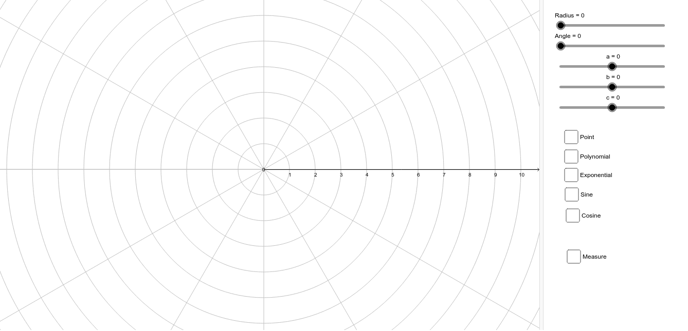
This example demonstrates the plotting and dynamic behavior of graphs in polar coordinates. Key math concepts include polar coordinates, function graphs, and parametric equations. Construction highlights involve the CurveCartesian command for Cartesian curve plotting, with parameters like Radius, Angle, and variables A, a, b, c, f, g, h, i, e. Suitable for high school and above students learning polar coordinates and function graphs, or for educational demonstrations.
GeoGebra Commands & Parameters
CurveCartesian((((a * t^(b)) + c) * cos(t)), (((a * t^(b)) + c) * sin(t)), t, 0, (10 * π)) → fCurveCartesian(((a * cos((b * t))) * cos(t)), ((a * cos((b * t))) * sin(t)), t, 0, (10 * π)) → gCurveCartesian(((a * sin((b * t))) * cos(t)), ((a * sin((b * t))) * sin(t)), t, 0, (10 * π)) → hCurveCartesian(((a * b^(t)) * cos(t)), ((a * b^(t)) * sin(t)), t, 0, (10 * π)) → iCurveCartesian((Radius * cos(t)), (Radius * sin(t)), t, 0, Angle) → e
AI Drawing Prompt Reference
Create a demonstration of the plotting and dynamic behavior of graphs in polar coordinates, including five different curves generated by polar coordinate equations, such as combinations of a*t^b*cos(t) and a*t^b*sin(t), a*cos(b*t)*cos(t) and a*cos(b*t)*sin(t), a*b^t*cos(t) and a*b^t*sin(t), and Radius*cos(t) and Radius*sin(t), to showcase the variety and changes in polar coordinate functions, suitable for high school and above students learning polar coordinates and function graphs.
The prompt above was compiled from the original drawing commands and is for reference only.