
Polar Area
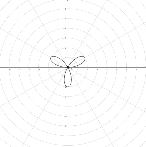
Loading the math board and drawing, please wait…
This example demonstrates the drawing of areas in the polar coordinate system. It involves basic concepts of polar coordinates, such as polar radius and angle. Using GeoGebra commands like CurveCartesian, Sequence, and Textfield, you can dynamically adjust parameters to observe the areas represented by different polar coordinate equations. Suitable for high school mathematics education, particularly for coordinate geometry and parametric equations.
GeoGebra Commands & Parameters
CurveCartesian((f(t) * cos(t)), (f(t) * sin(t)), t, a, b) → cSequence(c(i), i, a, b, d) → l1, {(0, 0), (2.4492935982947054E-16, -4.2423009548996277E-16), (4.898587196589417E-16, 8.484601909799253E-16), (-1.4695761589768238E-15, 3.5994234783884583E-31)}Sequence(Segment[(0, 0), Element[l1, i]], i, 1, n + 1) → l2, {0, 0, 0, 0}Textfield(f) → InputBox1Textfield(a) → InputBox2Textfield(b) → InputBox3Sequence(Circle[(0, 0), Element[l2, i]], i, 1, n + 1) → l3, {x² + y² = 0, x² + y² = 0, x² + y² = 0, x² + y² = 0}Sequence(Sector[Element[l3, i + 1], a + (i * d), a + (i * d) + d], i, 0, n - 1) → l4, {NaN, NaN, NaN}