
Periodic Function Action!
Loading the math board and drawing, please wait…
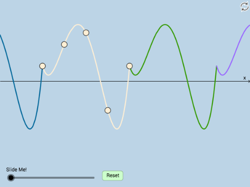
This example demonstrates how to create dynamic graphs of periodic functions using interactive geometry software, allowing users to modify function definitions. Key mathematical concepts include trigonometric functions, continuity, integral calculus, and secant lines. Construction involves GeoGebra commands such as Point, FitPoly, Vector, Translate, Dilate, and Segment with various objects. Suitable for high school students or college undergraduates learning trigonometric properties and geometric construction techniques.
GeoGebra Commands & Parameters
Point(x = (-a)) → APoint(x = ((-a)) / 2) → BPoint(x = 0) → CPoint(x = a / 2) → DFitPoly({A, B, C, D, E}, 4) → fVector(A, E) → uTranslate(g, u) → g_1Translate(g_1, u) → hTranslate(g, Vector[(-u)]) → g_2Translate(g_2, Vector[(-u)]) → pDilate(A, If[0 < b ≤ 1, 1 - b, 0], E) → A'Vector(A, A') → vSegment(A, A') → iTranslate(E, u) → E'Dilate(E, If[2 < b ≤ 3, 3 - b, 0], E') → E'_1Vector(E, E'_1) → wTranslate(g, w) → g_3Translate(A, w) → A'_1Translate(A', w) → A''Segment(A'_1, A'') → i'
AI Drawing Prompt Reference
Create a dynamic graph of a periodic function with an adjustable definition. Show continuity and integral calculus, and draw secant lines. Start by creating several points, then fit a polynomial function using these points. Next, use vectors to perform translation and dilation operations, generating multiple related graphical elements. Finally, connect some points to form segments, demonstrating the geometric properties and changes of the function.
The prompt above was compiled from the original drawing commands and is for reference only.