
Parameterized Curve and Locus Demo
Loading the math board and drawing, please wait…
In collections
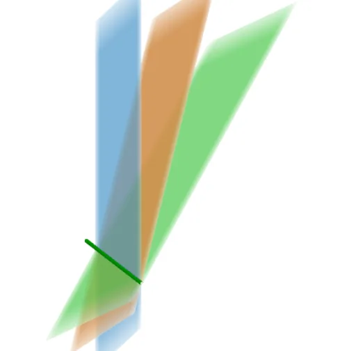
Systems of Three Linear Equations
This example dynamically demonstrates the locus of parametric equations, visually linking function graphs with geometric shapes. Core math concepts include parametric equations, locus, logarithmic functions, binomial distribution, cosine, and coordinate geometry. Construction highlights use of IntersectPath command for intersection points, combined with slider animations and text annotations via objects like a, b, f, c, d, e. Suitable for high school and above, aiding deep understanding and visualization of parametric equations and loci in mathematics education.
GeoGebra Commands & Parameters
IntersectPath(a, b) → fIntersectPath(a, c) → hIntersectPath(c, b) → i
AI Drawing Prompt Reference
Create a dynamic mathematical illustration showing the locus of parametric equations. Include two intersecting curves, one logarithmic and one cosine, crossing each other. Add a third auxiliary curve or line that intersects both, producing three distinct intersection points. Connect these points with a smooth path to form a moving locus that changes as a parameter varies. Include a slider control to adjust the parameter and text annotations explaining the relationship between the parametric equations and the locus. Emphasize the visual connection between function graphs and geometric shapes, suitable for educational demonstration.
The prompt above was compiled from the original drawing commands and is for reference only.