
Painted Cube 4x4x4
Loading the math board and drawing, please wait…
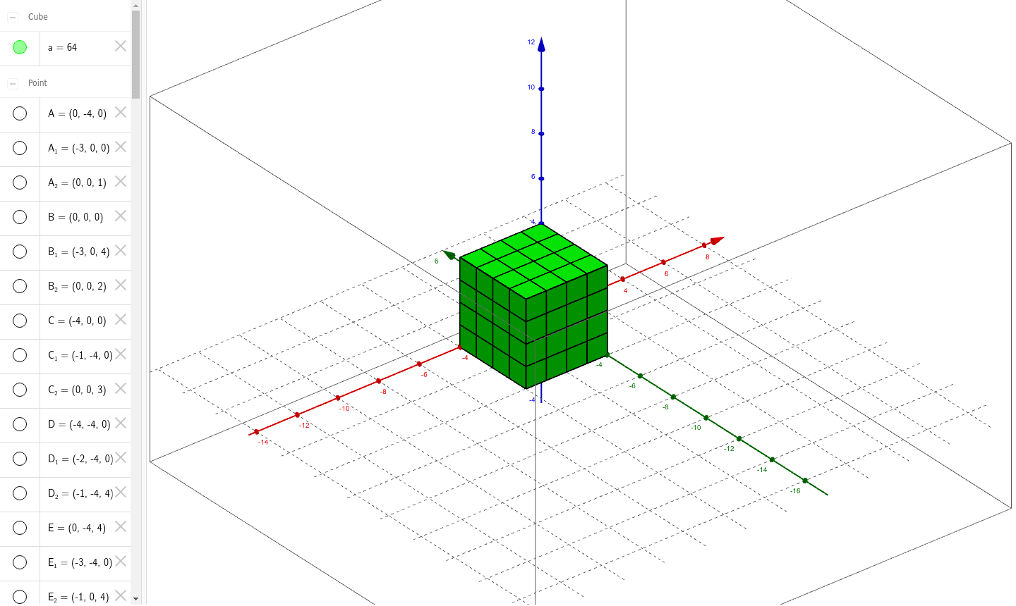
① This example demonstrates a 4×4×4 painted cube, allowing users to explore its three‑dimensional structure and symmetry through interactive geometry. ② The core mathematical concepts include solid geometry (vertices, faces, edges of a cube), translation transformations, planar symmetry, and the geometry of right triangles formed by the cube's diagonals. ③ The construction uses GeoGebra commands such as Point, Intersect, Cube, Segment, and PointIn to create vertices (A, B, C, …), face objects (faceABCD, …), and edge objects, enabling visualization of painted faces and measurement of small cube sections. ④ It is suitable for high‑school geometry classes or modeling projects, helping students understand spatial properties of solids and practice dynamic geometric exploration.
GeoGebra Commands & Parameters
Point(yAxis) → AIntersect(xAxis, zAxis) → BPoint(Circle[B, Distance[A, B], Segment[A, B]]) → CCube(A, B, C) → a, D, faceCDHG, faceEFGH, edgeAD, edgeAB, edgeBC, edgeCD, edgeAE, edgeDH, edgeEH, edgeEF, E, edgeBF, edgeFG, edgeCG, edgeGH, F, G, H, faceABCD, faceADHE, faceABFE, faceBCGFPoint(edgeAB) → IPoint(edgeEF) → JSegment(I, J) → bPoint(edgeAB) → KPoint(edgeEF) → LSegment(K, L) → cPointIn(faceABFE) → MPoint(edgeEF) → NSegment(M, N) → dPoint(edgeCD) → OPoint(edgeGH) → PSegment(O, P) → ePoint(edgeCD) → QPointIn(faceCDHG) → RSegment(Q, R) → fPoint(edgeCD) → SPoint(edgeGH) → TSegment(S, T) → gSegment(J, T) → hSegment(L, R) → iSegment(P, N) → jPoint(xAxis) → UPoint(edgeFG) → VSegment(U, V) → kPoint(xAxis) → WPointIn(faceBCGF) → ZSegment(W, Z) → lPointIn(faceBCGF) → B_1Segment(A_1, B_1) → mSegment(U, C_1) → nSegment(W, D_1) → pPoint(edgeAD) → E_1Segment(A_1, E_1) → qSegment(O, M) → rSegment(Q, K) → sSegment(S, I) → tPoint(edgeEH) → F_1Segment(C_1, F_1) → a_1Intersect(p, edgeAD) → G_1Point(edgeEH) → H_1Segment(D_1, H_1) → b_1Point(edgeEH) → I_1Segment(E_1, I_1) → c_1Point(zAxis) → J_1Point(edgeCG) → K_1Segment(J_1, K_1) → d_1Point(zAxis) → L_1Point(edgeCG) → M_1Segment(L_1, M_1) → e_1Point(edgeBF) → N_1Point(edgeCG) → O_1Segment(N_1, O_1) → f_1Point(edgeCG) → P_1Point(edgeDH) → Q_1Segment(P_1, Q_1) → g_1PointIn(faceCDHG) → R_1Point(edgeDH) → S_1Segment(R_1, S_1) → h_1Point(edgeCG) → T_1Point(edgeDH) → U_1Segment(T_1, U_1) → i_1Point(edgeAE) → V_1Segment(Q_1, V_1) → j_1PointIn(faceADHE) → W_1Segment(S_1, W_1) → k_1Point(edgeAE) → Z_1Segment(U_1, Z_1) → l_1Intersect(zAxis, f_1) → A_2Segment(Z_1, A_2) → m_1Point(zAxis) → B_2Segment(B_2, W_1) → n_1Point(zAxis) → C_2Segment(V_1, C_2) → p_1Intersect(edgeEH, a_1) → D_2Point(edgeFG) → E_2Segment(D_2, E_2) → q_1Intersect(edgeFG, l) → F_2Intersect(edgeEH, b_1) → G_2Segment(F_2, G_2) → r_1Intersect(edgeEH, c_1) → H_2Intersect(edgeFG, m) → I_2Segment(H_2, I_2) → s_1
AI Drawing Prompt Reference
Draw a 4×4×4 cube showing its vertices, edges, faces, and the internal grid of 64 smaller cubes. All six faces are painted and marked with equally spaced lines parallel to the edges, forming a 4×4 square grid on each face. Inside the cube, draw three sets of parallel cross‑sections along the three axes to create a 3D lattice. Also depict the space diagonals and the right triangles formed with face diagonals, illustrating translational and planar symmetry. The figure should display the full vertex‑edge‑face relationships of the solid, making the painted faces and small cube sections easy to locate.
The prompt above was compiled from the original drawing commands and is for reference only.