
Orbit of Planets 2
Loading the math board and drawing, please wait…
In collections
Complex Math
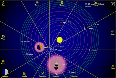
This example demonstrates the behavior of planetary orbits. It involves the concept of functions, particularly the parametric equations of orbits. Using GeoGebra commands such as Point, Segment, Polygon, Circle, and Intersect, you can dynamically observe the changes in planetary orbits. Suitable for high school mathematics education and learning.
GeoGebra Commands & Parameters
Point(b) → APoint(c) → BSegment(C, A) → dSegment(C, B) → fPoint(c) → DSegment(B, D) → iPoint(Circle[A, 1.4142135623730951]) → FSegment(A, F) → gSegment(A, F) → hPolygon(B, C, D) → poly1, d_1, b_1, c_1Segment(C, D) → d_hPoint(c) → EPoint(c) → GSegment(B, G) → τSegment(F, G) → nSlope(n) → mSlope(d_h) → m_1Circle(C, A) → kArea(k) → ePointIn(k) → PointkLine(H, f) → jIntersect(k, j, 2) → ISegment(C, I) → lLine(I, b) → pIntersect(p, d) → JSegment(C, J) → qSegment(J, I) → sPoint(s) → KSegment(C, K) → tSegment(I, F) → a_1Segment(J, A) → e_1Polygon(C, I, F, G, B) → poly2, c_2, i_1, f_1, g_1, b_2Name(o) → A1Name(u) → B1Name(a) → C1Point(k) → LCircle(M, N) → h_1Point(h_1) → OPoint(h_1) → PMidpoint(O, P) → QSegment(M, O) → j_1Segment(z_1, z_2) → k_1Vector(T, U) → vTranslate(z_1, v) → z_3Translate(z_2, v) → z_4Segment(z_3, z_4) → l_1Point(l_1) → VSegment(V, W) → n_1Segment(V, Z) → p_1Segment(V, A_1) → q_1Segment(V, B_1) → r_1Segment(V, C_1) → s_1Segment(V, D_1) → t_1Segment(V, E_1) → a_2Segment(V, F_1) → d_2Segment(V, G_1) → e_2Point(j_1) → H_1Circle(H_1, I_1) → f_2Circle(H_1, J_1) → g_2Circle(H_1, K_1) → h_2Circle(H_1, L_1) → k_2Circle(H_1, M_1) → p_2Circle(H_1, N_1) → q_2Circle(H_1, O_1) → r_2Point(h_1) → P_1Circle(H_1, P_1) → s_2Segment(V, Q_1) → i_2