Numerical Integration with Riemann Sums

Loading the math board and drawing, please wait…

2019-03-09 05:42

Function Calculus Integral

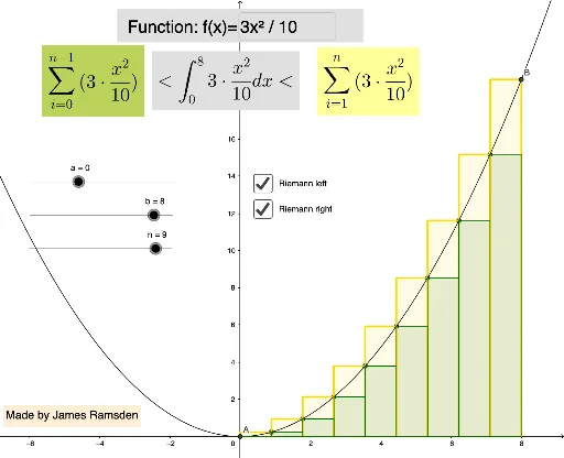
This example demonstrates numerical integration using Riemann sums. Key mathematical concepts include definite integrals and approximating the integral of a function. Using GeoGebra commands like Sequence, Sum, and Polygon, users can dynamically adjust intervals and partition points to observe the approximation of Riemann sums. Suitable for high school math education and learning calculus concepts.

GeoGebra Commands & Parameters

Sequence(a + (i * (b - a) / n), i, 0, n) → list1
Sequence((Element[list1, i], f(Element[list1, i])), i, 1, n + 1) → list5
Sequence(Polygon[(Element[list1, i], 0), Element[list5, i], Element[list5, i] + ((b - a) / n, 0), (Element[list1, i + 1], 0)], i, 1, n) → list7
Sum(list7) → p
Textfield(f) → inputBox1
Sequence(Polygon[(Element[list1, i], 0) - ((b - a) / n, 0), Element[list5, i] - ((b - a) / n, 0), Element[list5, i], (Element[list1, i], 0)], i, 2, n + 1) → list6
Polygon(C, D, E, F) → q1, c, d, e, f_1

AI Drawing Prompt Reference

Draw the Riemann sum approximation of the function f over the interval [a, b]. First, generate n equally spaced points, then draw rectangles with their bases on the x-axis and heights equal to the function values at these points. Finally, calculate the total area of these rectangles as an approximation of the integral of the function over the interval.

The prompt above was compiled from the original drawing commands and is for reference only.