Numerical Integration and Projectile Trajectories

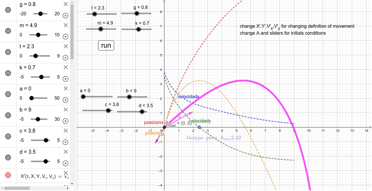
This GeoGebra example demonstrates projectile motion simulated via numerical integration, showing the flight path, velocity components, and maximum height under gravity. Core mathematical concepts include numerical solution of ordinary differential equations (e.g., Euler or Runge-Kutta methods), vector decomposition, parametric curves, and the application of integrals in physics. Construction highlights: the NSolveODE command solves the motion differential equations, while Vector, Locus, PathParameter, and Element commands visualize velocity vectors and the trajectory. Interactive sliders and a button allow users to adjust initial speed and launch angle, with real-time updates of position, velocity, and other metrics. Suitable for high school to undergraduate physics and mathematics courses, this example helps learners grasp the practical meaning of numerical integration and differential equations, as well as parametric modeling of projectile motion.