Normal Distribution with Variable Tail Areas

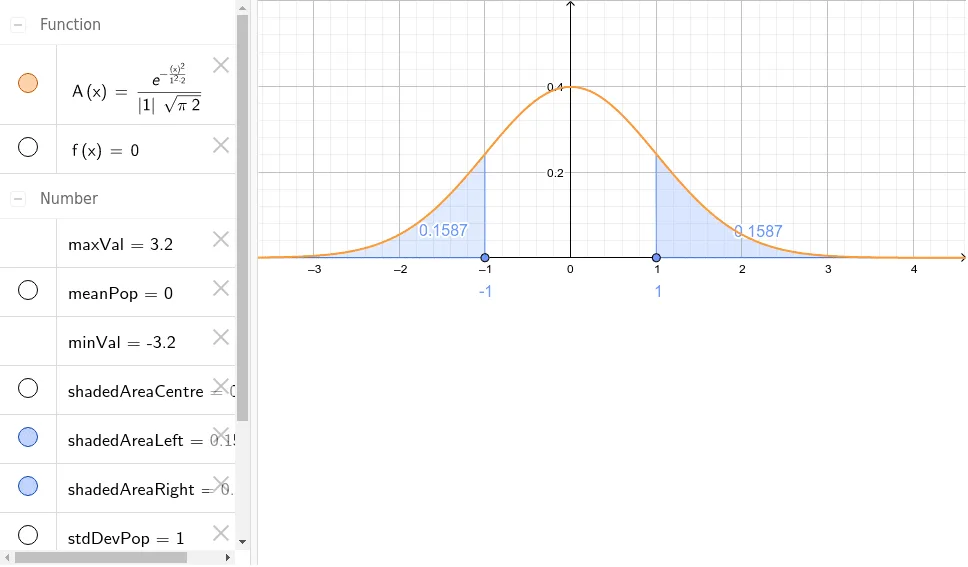
This example demonstrates how the areas under the tails of a normal distribution change as parameters vary. Key math concepts include normal distribution, probability density function, integration, and hypothesis testing. Construction highlights involve using commands like Normal for the curve, Point for creating points, and IntegralBetween for calculating areas, with sliders and objects such as meanPop and stdDevPop to manipulate parameters. The visualization shows shaded areas (left, right, center) corresponding to different regions. Suitable for high school and above students/teachers learning probability distributions and statistical inference.