Normal Distribution with Variable Areas in Left Tail

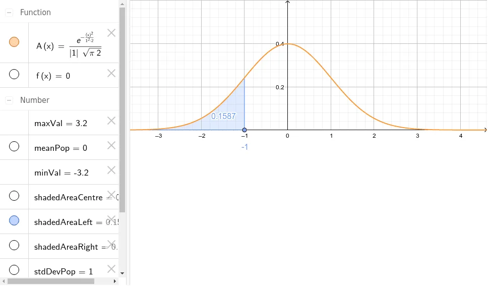
This example demonstrates how the area under the left tail of a normal distribution changes with varying parameters. Key math concepts include normal distribution, probability density function, definite integral, and symmetry. Construction highlights involve using commands like Normal, Point, and IntegralBetween with objects such as meanPop (mean), stdDevPop (standard deviation), A (area variable), and P (probability). Suitable for high school and above students studying probability & statistics and calculus.