
Normal Distribution with Variable Areas in Right Tail
Loading the math board and drawing, please wait…
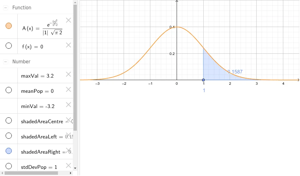
This example demonstrates how the area under the right tail of a normal distribution changes with varying parameters. Key math concepts include normal distribution, integral calculus, and probability & statistics. It is constructed using commands like Normal, Point, and IntegralBetween, with objects such as meanPop, stdDevPop, A, etc. Suitable for high school students and learners needing to understand probability and calculus concepts.
GeoGebra Commands & Parameters
Normal(meanPop, stdDevPop, x) → APoint(xAxis) → PPoint(xAxis) → QIntegralBetween(A, f, x(P), x(Q)) → shadedAreaCentreIntegralBetween(A, f, x(Q), 100) → shadedAreaRightIntegralBetween(A, f, -100, x(P)) → shadedAreaLeft
AI Drawing Prompt Reference
Draw a normal distribution curve with two points on the x-axis representing the integral limits. Calculate and display the area from the lower limit to the center point, as well as the areas from the center point to positive infinity and from negative infinity to the lower limit, to show how the right tail area changes with varying parameters.
The prompt above was compiled from the original drawing commands and is for reference only.