
Normal Distribution GeoGebra Demo
Loading the math board and drawing, please wait…
In collections
Pearson Maths A level Statistics and Mechanics 2
Pearson Maths A level Statistics and Mechanics 2
Pearson Maths A level Statistics and Mechanics 2
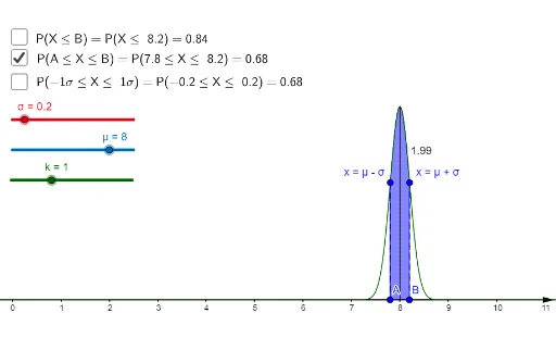
This example demonstrates the probability density function of the normal distribution and its properties. Key math concepts include probability & statistics, integral, function graphing, and parameter adjustment. GeoGebra commands used are Sequence, Point, Integral, Intersect, OrthogonalLine, Segment, and Vector. Suitable for high school and above students to learn the geometric meaning and calculation of the normal distribution.
GeoGebra Commands & Parameters
Sequence(Segment[(-100, i), (100, i)], i, -50, 50, 1) → list2Sequence(Segment[(i, -100), (i, 100)], i, -50, 50, 1) → list4Point(g) → APoint(g) → BIntegral(f, x(A), x(B)) → bIntersect(f, i, (7.8, 1.2098536225957157)) → DIntersect(f, h, (8.2, 1.2098536225957213)) → EIntegral(f, -30, x(B)) → aOrthogonalLine(D, g) → jOrthogonalLine(E, g) → lIntersect(j, g) → CIntersect(f, l, (8.2, 1.2098536225957213)) → FIntersect(l, g) → GSegment(D, C) → mSegment(E, G) → nOrthogonalLine(A, g) → pOrthogonalLine(B, g) → qIntersect(f, p, (7.7958398050734035, 1.1846910986063952)) → HIntersect(f, q, (8.196026449007489, 1.233887519690266)) → ISegment(H, A) → rSegment(I, B) → sIntegral(f, ((-k) * σ) + μ, (k * σ) + μ) → oIntersect(f, f_1, (8, 1.9947114020071635)) → JPoint(f_1) → KIntersect(j, f_1) → LIntersect(g, f_1) → MVector(M, K) → vSegment(M, J) → g_1