Normal Distribution Demo: Integration and Probability

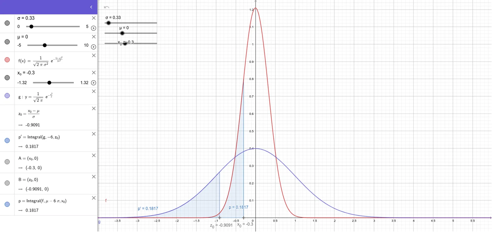
This GeoGebra example dynamically illustrates the normal distribution curve and its integral area, showing the relationship between the probability density function and cumulative probability. Core mathematical concepts include normal distribution (parameters μ and σ), probability density function, definite integral for area, expected value, and standard normal transformation. Construction highlights: the Integral command computes the area under the curve from negative infinity to x₀, with objects σ, μ, f (density function), x₀ (upper limit), g (auxiliary function), z_0 (standardized variable), p' (probability value), A, B (area regions), and p (probability point). Suitable for high school and college statistics and calculus courses, this demo helps students understand normal distribution properties, z-scores, and probability calculations. It serves as an interactive teaching tool for instructors or a self-exploration resource for learners.