
Normal Distribution by Mark Willis
Loading the math board and drawing, please wait…
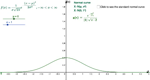
This example demonstrates the probability density function of the normal distribution. The normal distribution is a fundamental concept in probability and statistics, characterized by a bell-shaped curve. By adjusting parameters μ (mean) and σ (standard deviation), the shape of the curve can be observed. This example uses the Normal command to draw the normal distribution curve, suitable for high school and above students to learn about probability and statistics.
GeoGebra Commands & Parameters
Normal(0, 1, x, false) → fNormal(μ, σ, x, false) → gLaTeX(g, true, true) → text1LaTeX(f, true, true) → text2
AI Drawing Prompt Reference
Draw a coordinate system with two normal distribution curves. The first curve is a standard normal distribution with mean 0 and standard deviation 1, showing a symmetric bell shape. The second curve uses adjustable mean and standard deviation parameters, with its shape varying accordingly. Both curves are plotted as probability density functions, not cumulative probabilities. Next to each curve, display its corresponding function expression in LaTeX format for clear comparison between the standard and parameterized normal distributions. The layout should emphasize the curve shapes and how parameters affect the distribution.
The prompt above was compiled from the original drawing commands and is for reference only.