
Normal Curve of Binomial Distribution
Loading the math board and drawing, please wait…
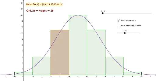
This example demonstrates how the binomial distribution approximates a normal curve with a large number of trials. Key mathematical concepts include binomial distribution and probability statistics. Using commands like If, Sequence, Max, Min, Polygon, Element, and Text, the binomial distribution's probability histogram is constructed and observed to approach a normal curve as the number of trials increases. Suitable for high school and above students or teachers.
GeoGebra Commands & Parameters
If(i, 0, 1) → nSequence(nCr[a, i], i, 0, a, 1) → l1Max(l1) → bSequence(Element[l1, i] / 2^(a), i, 1, a + 1, 1) → l2Max(l2) → hMin(l1) → cSequence((i, 0), i, 0, a) → l3Sequence((i - 1, Element[l1, i]), i, 1, a + 1) → l4Sequence(Polygon[Element[l3, i] - (0.5, 0), Element[l3, i] + (0.5, 0), Element[l4, i] + (0.5, 0), Element[l4, i] - (0.5, 0)], i, 1, a + 1) → l5Max(l2) → eSequence((i / o - a / 2 / o, 0), i, 0, a) → l6Sequence(Polygon[Element[l6, i] - (1 / ((2 * o)), 0), Element[l6, i] + (1 / ((2 * o)), 0), Element[l6, i] + (1 / ((2 * o)), 0) + (0, Element[l2, i]), Element[l6, i] - (1 / ((2 * o)), 0) + (0, Element[l2, i])], i, 1, a + 1) → l7Sequence(nCr[a, i], i, 0, a, 1) → l1_1Max(l1_1) → b_1Min(l1_1) → c_1Polygon(Element[l3, r_2] - (0.5, 0), Element[l3, r_2] + (0.5, 0), Element[l4, r_2] + (0.5, 0), Element[l4, r_2] - (0.5, 0)) → q1, l, p, q, r_1Polygon(Element[l6, r_2] - (1 / ((2 * o)), 0), Element[l6, r_2] + (1 / ((2 * o)), 0), Element[l6, r_2] + (1 / ((2 * o)), 0) + (0, Element[l2, r_2]), Element[l6, r_2] - (1 / ((2 * o)), 0) + (0, Element[l2, r_2])) → q2, s, t, f_1, g_1Element(l1, r_2) → uElement(l2, r_2) → wText("C(" + a + "," + r + ") = height =" + q1, A, true, true) → text2Sequence(nCr[a, i], i, 0, a, 1) → l1_2Max(l1_2) → b_2Sequence(Element[l1_2, i] / 2^(a), i, 1, a + 1, 1) → l2_1Max(l2_1) → h_1Min(l1_2) → c_2Max(l2_1) → e_1Element(l1_2, r_3) → u_1Element(l2_1, r_3) → w_1