
Normal Approximation to the Binomial with Continuity Correction
Loading the math board and drawing, please wait…
In collections
JHU EN.550.311 Spring 2014
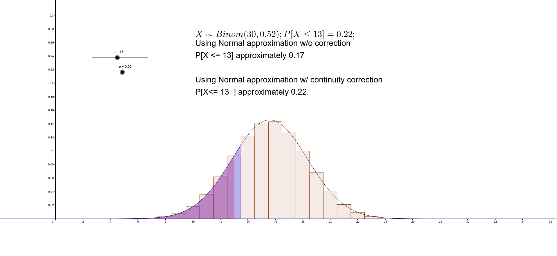
This example demonstrates the impact of the continuity correction on the Normal approximation to the Binomial distribution. It covers core concepts like binomial distribution, normal distribution, continuity correction, and probability calculation. Constructed using GeoGebra commands BinomialDist, Normal, involving objects such as n, p, a, b, f, t, pTrue, c, d, pApproxNC, pApproxCC, g, e, h, i, text1, text2. Suitable for high school and above students learning probability and statistics for understanding approximation methods.
GeoGebra Commands & Parameters
BinomialDist(n, p) → aBinomialDist(n, p, 5, true) → bBinomialDist(n, p, t, true) → pTrueNormal(n * p, sqrt(n * p * (1 - p)), t) → dNormal(n * p, sqrt(n * p * (1 - p)), t) → pApproxNCNormal(n * p, sqrt(n * p * (1 - p)), t + 0.5) → pApproxCC
AI Drawing Prompt Reference
Draw a binomial distribution graph showing true probability and normal approximation, including both uncorrected and continuity correction cases. First plot the probability mass function of the binomial distribution, then draw the corresponding normal distribution curves for both uncorrected and continuity-corrected approximations. Use different colors for the curves and label key parameters and probability values to show the impact of continuity correction on the approximation.
The prompt above was compiled from the original drawing commands and is for reference only.