
Normal Approximation to the Binomial Distribution by strong1kaden
Loading the math board and drawing, please wait…
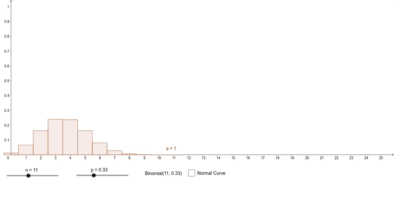
This example demonstrates the normal approximation to the binomial distribution by adjusting the parameters n and p. Key mathematical concepts include binomial distribution and normal distribution. The BinomialDist and Normal commands in GeoGebra are used to construct the graph. Suitable for high school mathematics education and students learning probability and statistics.
GeoGebra Commands & Parameters
BinomialDist(n, p) → aNormal((n * p), sqrt(((n * p) * (1 - p))), x, false) → f
AI Drawing Prompt Reference
Create a graph illustrating the normal approximation to the binomial distribution. First, plot the binomial probability mass function as discrete points based on the number of trials and success probability. Then, draw a continuous normal density curve with mean equal to the product of trials and success probability, and standard deviation equal to the square root of that product times the failure probability. Adjust the parameters to show how the curve approximates the discrete points. Include axes, the discrete point series, and the smooth curve, emphasizing their shape similarity.
The prompt above was compiled from the original drawing commands and is for reference only.