Normal Approximation to the Binomial Distribution (1)

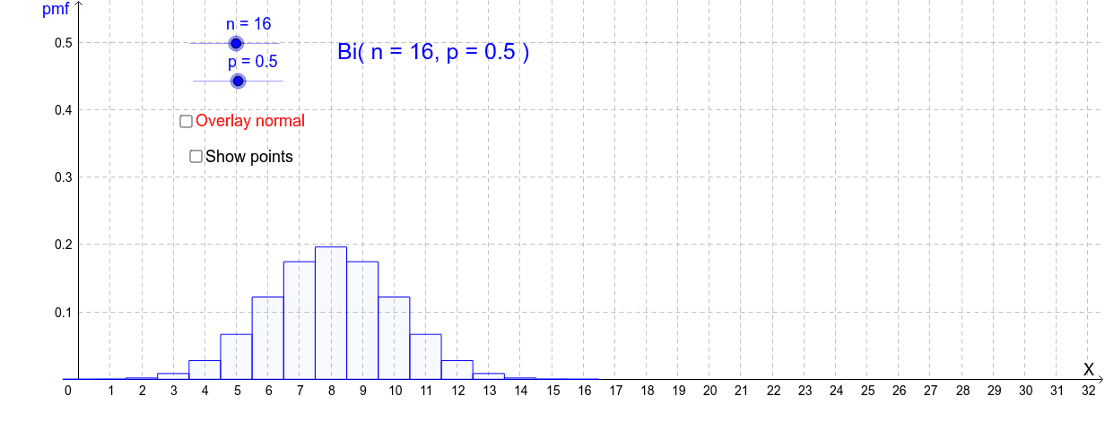
This example demonstrates the normal approximation to the binomial distribution. By simulating random samples from a binomial distribution and plotting the frequency histogram alongside the normal distribution curve, it visually illustrates how the normal distribution approximates the binomial distribution. Key mathematical concepts involved include binomial distribution, normal distribution, expected value, and standard deviation. The construction utilizes GeoGebra commands and objects such as Point, If, BinomialDist, BarChart, Integral, with sliders to dynamically adjust parameters n and p to observe the goodness of fit between the normal curve and the histogram. Suitable for high school and above students learning about the central limit theorem in probability and statistics.