
Normal Approximation of Binomial Distribution
Loading the math board and drawing, please wait…
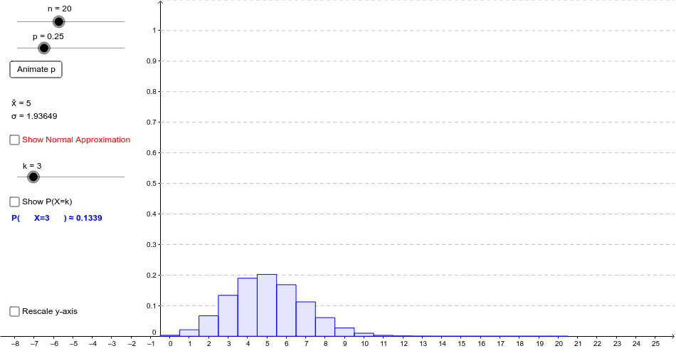
This example illustrates the normal approximation of the binomial distribution for 1 ≤ n ≤ 50, displaying the discrete probability mass function alongside its continuous normal approximation. Users can adjust the success probability p via sliders, and the mean μ and standard deviation σ are computed and shown dynamically. Key mathematical concepts include the binomial distribution, normal distribution, central limit theorem, probability mass versus density functions. The construction uses BinomialDist for probabilities, Normal for the curve, If for conditional display, Polygon for shading, and objects such as p, n, shownormdist, showPk, animatep, etc., to enable interactive animation. It is suitable for high‑school (grades 12‑13) and early college students in statistics and data science courses.
GeoGebra Commands & Parameters
Normal((n * p_-), sqrt(((n * p_-) * (1 - p_-))), x) → f_-Normal((n * p_+), sqrt(((n * p_+) * (1 - p_+))), x) → f_+Normal(μ, σ, x) → fIf(n ≤ 25, 26, n + 1) → xmaxBinomialDist(n, p) → binomplotIf(rescale, If[p ≟ 0, f_+((n * p_+)), If[p ≟ 1, f_-((n * p_-)), f(μ)]], 1) → ymaxBinomialDist(n, p) → binomplotbordIf((1.1 * ymax) ≤ 0.5, 0.05, If[0.5 ≤ (1.1 * ymax) ≤ 2, 0.1, If[2 ≤ (1.1 * ymax) ≤ 4, 0.2, If[4 ≤ (1.1 * ymax) ≤ 8, 0.5, If[(1.1 * ymax) > 8, 1]]]]) → ygriddistZip(Ray[A, B], A, Sequence[((-0.5), (ygriddist * i)), i, 1, ygridnum], B, Sequence[(0, (ygriddist * i)), i, 1, ygridnum]) → ygridPolygon((k - 0.5, 0), (k - 0.5, BinomialDist[n, p, k, false]), (k + 0.5, BinomialDist[n, p, k, false]), (k + 0.5, 0)) → binomkplot, binomkplota, binomkplotb, binomkplotc, binomkplotd
AI Drawing Prompt Reference
Create an interactive plot that shows the binomial probability mass function for a variable number of trials n (1 to 50) and success probability p, together with its normal approximation curve. The figure displays the mean μ and standard deviation σ computed from n and p, a continuous normal density curve, and rectangular bars for each integer k spanning from k‑0.5 to k+0.5 with height equal to the binomial probability. The x‑axis range is fixed at 26 when n ≤ 25 and expands with n otherwise; the y‑axis scales automatically and grid lines adapt to the maximum probability. Sliders control n, p, and toggles for showing the normal curve and individual probability bars.
The prompt above was compiled from the original drawing commands and is for reference only.