
Non Uniform Linear Motion with Constant Acceleration
Loading the math board and drawing, please wait…
In collections
Prof. Stick's Mostly Good Guide to Physics
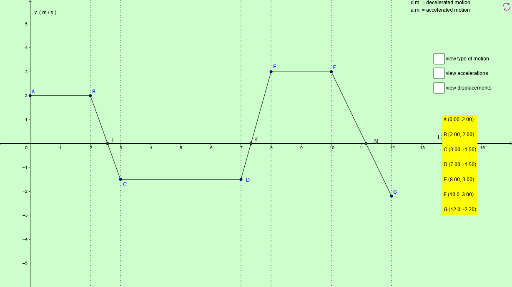
This example illustrates the relationship between non-uniform linear motion and constant acceleration. Key mathematical concepts include linear motion, acceleration, and velocity. Using GeoGebra commands such as Point, Polygon, Segment, etc., the position, velocity, and acceleration curves of a moving object can be constructed. Suitable for high school physics and mathematics education.
GeoGebra Commands & Parameters
Point(yAxis) → A_1Point(yAxis) → B_1Polygon(A_1, C_1, D_1, B_1) → poli1, a_1, c, d, b_1Point(b_1) → APointIn(poli1) → FPointIn(poli1) → GPointIn(poli1) → BPointIn(poli1) → CPointIn(poli1) → DPointIn(poli1) → ESegment(A, B) → eSegment(B, C) → fSegment(C, D) → gSegment(D, E) → hSegment(E, F) → iSegment(F, G) → jIntersect(e, xAxis) → HIntersect(f, xAxis) → IIntersect(g, xAxis) → JIntersect(h, xAxis) → KIntersect(i, xAxis) → LIntersect(j, xAxis) → MSlope(e) → A1Slope(f) → A2Slope(g) → A3Slope(h) → A4Slope(i) → A5Slope(j) → A6Segment((x(A), A1), (x(B), A1)) → lSegment((x(B), A2), (x(C), A2)) → n_2Segment((x(D), A3), (x(C), A3)) → pSegment((x(D), A4), (x(E), A4)) → qSegment((x(F), A5), (x(E), A5)) → rSegment((x(F), A6), (x(G), A6)) → sCurveCartesian(t, (y(A) * t) + (A1 * t^(2) / 2), t, 0, x(B)) → vCurveCartesian(t, spo1 + (y(B) * (t - x(B))) + (A2 * (t - x(B))^(2) / 2), t, x(B), x(C)) → uCurveCartesian(t, spo1 + spo2 + (y(C) * (t - x(C))) + (A3 * (t - x(C))^(2) / 2), t, x(C), x(D)) → wCurveCartesian(t, spo1 + spo2 + spo3 + (y(D) * (t - x(D))) + (A4 * (t - x(D))^(2) / 2), t, x(D), x(E)) → zCurveCartesian(t, spo1 + spo2 + spo3 + spo4 + (y(E) * (t - x(E))) + (A5 * (t - x(E))^(2) / 2), t, x(E), x(F)) → c_1CurveCartesian(t, spo1 + spo2 + spo3 + spo4 + spo5 + (y(F) * (t - x(F))) + (A6 * (t - x(F))^(2) / 2), t, x(F), x(G)) → d_1OrthogonalLine(B, xAxis) → e_1OrthogonalLine(C, xAxis) → f_1OrthogonalLine(D, xAxis) → g_1OrthogonalLine(E, xAxis) → h_1OrthogonalLine(F, xAxis) → i_1Max(A10, 0, x(B)) → B10Max(A11, x(B), x(C)) → B11Max(A12, x(C), x(D)) → B12Max(A13, x(D), x(E)) → B13Max(A14, x(E), x(F)) → B14Max(A15, x(F), x(G)) → B15Min(A10, 0, x(B)) → D10Min(A11, x(B), x(C)) → D11Min(A12, x(C), x(D)) → D12Min(A13, x(D), x(E)) → D13Min(A14, x(E), x(F)) → D14Min(A15, x(F), x(G)) → D15Max(lista2) → D1Min(lista3) → D2Min(lista1) → A7Max(lista1) → A8Point(p) → NPoint(n_2) → OPoint(l) → PPoint(r) → QPoint(s) → RPoint(q) → SPoint(v) → TPoint(u) → UPoint(w) → VPoint(z) → WPoint(c_1) → ZPoint(d_1) → E_1If(m ∧ (¬n), Min[A7, -5] - 1, If[n ∧ (¬m), Min[D2, -5] - 1, If[m ∧ n, Min[lista5] - 1, -6]]) → yminIf(m ∧ (¬n), Max[A8, 5] + 1, If[n ∧ (¬m), Max[D1, 5] + 1, If[m ∧ n, Max[lista4] + 1, 6]]) → ymaxOrthogonalLine(G, xAxis) → b
AI Drawing Prompt Reference
Draw a graph illustrating the relationship between non-uniform linear motion and constant acceleration. Start by creating a pentagon, then place six points on it and connect these points with line segments. Calculate the slope of each segment and draw five parallel line segments based on these slopes. Finally, use the segments and the pentagon to construct velocity and acceleration curves, showcasing the characteristics of non-uniform linear motion.
The prompt above was compiled from the original drawing commands and is for reference only.