
Nature of Critical Points of Function f(x, y): Local Max/Min and Saddle (1)
Loading the math board and drawing, please wait…
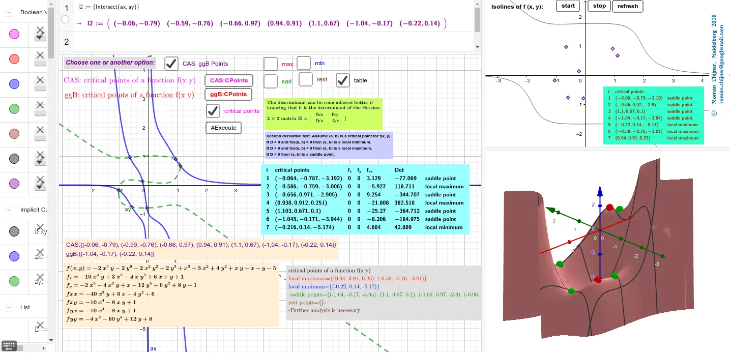
This example demonstrates the nature of critical points of a function f(x, y), including local maxima, local minima, and saddle points. Key mathematical concepts include derivatives and second derivatives. Using commands like Simplify and ImplicitCurve, the construction shows the critical points of the function and uses text rotation to illustrate different scenarios. Suitable for university calculus courses.
GeoGebra Commands & Parameters
Simplify(Derivative[f, x, 1]) → fxSimplify(Derivative[f, y, 1]) → fyImplicitCurve(fx(x, y)) → axImplicitCurve(fy(x, y)) → aySimplify(Derivative[fx, x, 1]) → fxxSimplify(Derivative[fx, y, 1]) → fxySimplify(Derivative[fy, y, 1]) → fyySimplify(Derivative[fy, x, 1]) → fyxZip({{fxx(a), fxy(a)}, {fyx(a), fyy(a)}}, a, l1) → MZip(Determinant[a], a, M) → DZip(fxx(a), a, l1) → f_{xx}Sequence(If[D(i) > 0, If[f_{xx}(i) > 0, "local minimum", "local maximum"], If[(D(i) * f_{xx}(i)) ≟ 0, "?", "saddle point"]], i, 1, Length[l1]) → l4Zip((x(a), y(a), f(a)), a, l1) → l5Zip(fx(a), a, l1) → lfxZip(fy(a), a, l1) → lfyTableText(Append["i", 1…Length[l1]], Append["critical points", l5], Append["f_{x}", lfx], Append["f_{y}", lfy], Append["f_{xx}", f_{xx}], Append["Det", D], Append["", l4], "v") → text1LaTeX(f, true) → text2Sequence(If[D(i) > 0, If[f_{xx}(i) > 0, 1, 2], If[D(i) ≟ 0, -5, -1]], i, 1, Length[l1]) → l4aSort(l5, l4a) → l5aSort(l1, l4a) → l1aLength(lmax) → lämaxLength(lmin) → läminLength(lsad) → läsadSort(l4, l4a) → l4aaTableText(Append["i", 1…Length[l1]], Append["critical points", l5a], Append["", l4aa], "v") → text1aLength(lq) → läqImplicitCurve(f(x, y) - z0) → IFxyZip((x(a), y(a)), a, lsad) → lsad_2Zip((x(a), y(a)), a, lq) → lq_2Zip((x(a), y(a)), a, lmax) → lmax_2Zip((x(a), y(a)), a, lmin) → lmin_2Max(z(lmax)) → maxMax(z(lmin)) → minRotateText(txt1, 90°) → txt2