Moving Functions: Graph Transformations with Coordinates

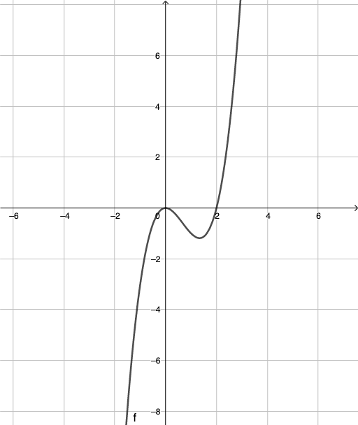
This example demonstrates how “moving functions” changes the graph in the coordinate plane: when a function is translated or adjusted according to a transformation rule, its graph shifts accordingly while preserving the overall shape correspondence. Key mathematical ideas include function graph transformations (translation/movement), coordinate-geometry interpretation, and the notion of congruence/corresponding figures under rigid transformations. From the construction summary (“objects: f”), the construction centers on defining or using a function object f as the primary object to be moved, then applying the intended transformation to generate and visualize the moved graph and its relation to the original. Suitable for middle-school algebra and coordinate-geometry instruction, and useful for interactive classroom demos where students can explore how transformation rules produce predictable graph movement.