
Monte Carlo Pi Estimation
Loading the math board and drawing, please wait…
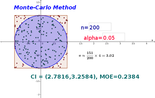
This example demonstrates the Monte Carlo method to estimate the value of Pi by randomly throwing darts inside a unit square and calculating the ratio of darts that land inside a unit circle. Key mathematical concepts include probability & statistics, geometric probability, frequency distribution, and confidence intervals. It utilizes GeoGebra commands like Sequence, Sum, Polygon, Zip, InverseNormal, and Textfield, along with objects such as alpha, n, darts, f, success, phat, sd. Suitable for high school students and above learning probability statistics and Monte Carlo methods, or for educational demonstrations.
GeoGebra Commands & Parameters
Sequence(((2 * random()) - 1, (2 * random()) - 1), k, 1, n) → dartsSum(Zip[f(A), A, darts]) → successPolygon(A, B, C, D) → border, a, b, c, dZip(f(A), A, darts) → junkSequence(If[Element[junk, k], Element[darts, k]], k, 1, n) → list1InverseNormal(phat, sd, (0.5 * alpha)) → cilowInverseNormal(phat, sd, 1 - (0.5 * alpha)) → cihighTextfield(n) → inputBox1Textfield(alpha) → inputBox2
AI Drawing Prompt Reference
Create a unit square and a unit circle. Randomly generate points inside the square and count how many fall inside the circle to estimate Pi. Display the points that fall inside the circle in a different color. Show the estimated value of Pi and the confidence interval based on the ratio of points inside the circle. Start by drawing the square and circle, then generate random points, count the ones inside the circle, and finally display the estimation and confidence interval next to the graph.
The prompt above was compiled from the original drawing commands and is for reference only.