Monte Carlo Pi Estimation with Confidence Interval Visualization

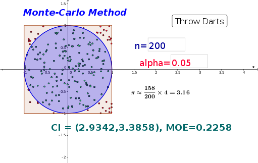
This GeoGebra example demonstrates the Monte Carlo method for estimating π by randomly throwing darts into a square and counting those falling inside an inscribed circle. It visualizes how the estimate converges and displays a confidence interval that narrows as the sample size increases. Core mathematical concepts include geometric probability, the law of large numbers, normal approximation to the binomial distribution, and confidence interval construction. The construction uses commands such as Sequence to generate random points, Sum to count successes, Polygon for the square and circle, Zip and InverseNormal to compute interval bounds, Textfield and inputBox for interactive parameters, and a button to rerun the simulation. Suitable for high school to undergraduate statistics courses, it helps learners grasp the randomness of simulation, the trade-off between accuracy and sample size, and the interpretation of confidence intervals in practice.