Modeling with Polynomial Functions by Aimee Haygood

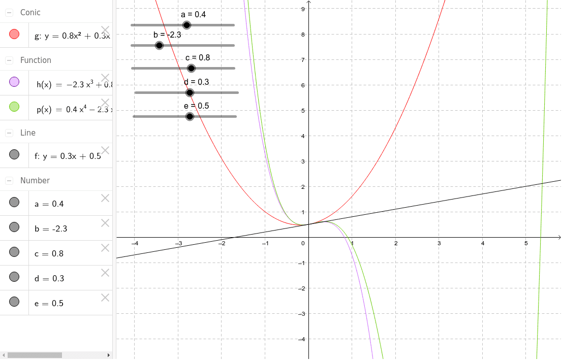
This GeoGebra example demonstrates how to model a set of data points using polynomial functions, allowing users to adjust coefficients to fit the curve to the scatter plot and observe the goodness of fit. Core mathematical concepts include polynomial functions, curve fitting, expected value, statistical correlation, and geometric elements such as rhombus and logarithmic functions. The construction uses objects a, b, c, d, e, f, h, p, and g, which likely represent polynomial coefficients, data points, fitted curves, and auxiliary geometric constructions. Users can manipulate sliders or input commands to dynamically update the polynomial model. This resource is suitable for high school or introductory college students learning function modeling, statistics, and data analysis, as well as for teachers demonstrating polynomial regression principles.