
Modeling with Polynomial Functions
Loading the math board and drawing, please wait…
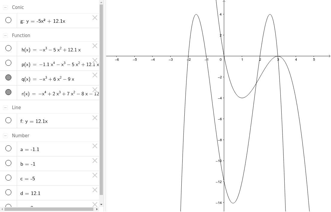
This example demonstrates how to use GeoGebra to construct polynomial function models and visualize their graphs and properties. Core math concepts include polynomial functions, function graphs, optimization problems, and analytical geometry. Construction highlights involve GeoGebra commands/objects like a, b, c, d, e, f, h, p, g, q, r, used for defining function parameters, plotting graphs, and calculating/displaying extrema. Suitable for high school and above learners to understand polynomial function applications and optimization.
GeoGebra Commands & Parameters
Numeric a(-1.1)Numeric b(-1)Numeric c(-5)Numeric d(12.1)Numeric e(0)y = (d * x) + eh(x) = (b * x^(3)) + (c * x^(2)) + (d * x) + ep(x) = (a * x^(4)) + (b * x^(3)) + (c * x^(2)) + (d * x) + ey = (c * x^(2)) + (d * x) + eq(x) = (-x^(3)) + (6 * x^(2)) - (9 * x)r(x) = (-x^(4)) + (2 * x^(3)) + (7 * x^(2)) - (8 * x) - 12
AI Drawing Prompt Reference
Draw the graphs of four polynomial functions: a linear function passing through the origin, a cubic function with two extrema, a quartic function, and another cubic function. Highlight the intersection points and extrema of these functions.
The prompt above was compiled from the original drawing commands and is for reference only.