
Measures of Central Tendency for Two Data Sets
Loading the math board and drawing, please wait…
In collections
Statistics and Probability with Mr Downes
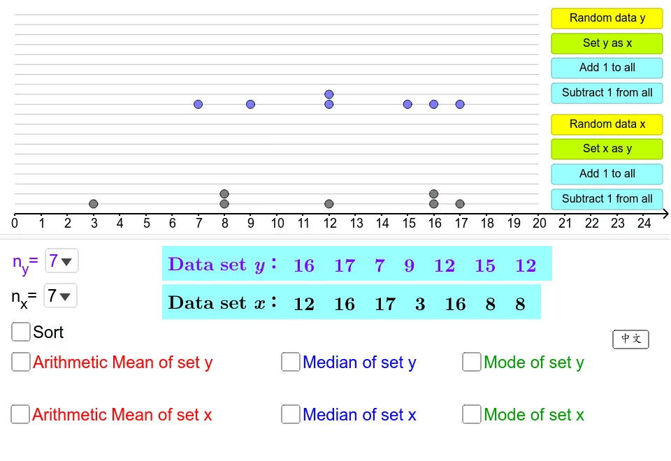
This GeoGebra example demonstrates the calculation and visualization of measures of central tendency (mean, median, mode) for two data sets, using boxplots to represent data distribution. Core mathematical concepts include descriptive statistics, central tendency measures, data sorting, and frequency analysis. The construction employs GeoGebra commands such as Sequence, Point, Sort, Mean, Median, Mode, Frequency, Flatten, Shuffle, Segment, and Zip, along with objects like sorted lists, meanX, and box1, to create interactive plots. It is suitable for high school or introductory college statistics courses, providing an engaging way to teach data analysis and graphical representation.
GeoGebra Commands & Parameters
SelectedElement(listNx) → nXSequence(Segment[(0, i), (20, i)], i, seperation, (20 * seperation), seperation) → listGridPoint(listGrid) → APoint(listGrid) → BPoint(listGrid) → CPoint(listGrid) → DPoint(listGrid) → EPoint(listGrid) → FPoint(listGrid) → GPoint(listGrid) → HPoint(listGrid) → IPoint(listGrid) → JSort(listDataX) → listDataXsortedMean(listDataX) → meanXIf(nX ≥ 11, 0.7, If[nX ≥ 9, 0.85, 1]) → scaleMedian(listDataX) → medianXRay((0, 0), (1, 0)) → bMode(listDataX) → listModeXSequence(Random[0, 20], i, 1, nX) → listRandXFrequency(listRandX) → listFreqXSort(listRandX) → listRandSortXFlatten(Zip[Sequence[(seperation * i), i, 1, k], k, listFreqX]) → listHeightXShuffle(Zip[(h, k), h, listRandSortX, k, listHeightX]) → listPositionXPoint(listGrid) → KPoint(listGrid) → LPoint(listGrid) → MPoint(listGrid) → NPoint(listGrid) → OPoint(listGrid) → PPoint(listGrid) → QPoint(listGrid) → RPoint(listGrid) → SPoint(listGrid) → TSelectedElement(listNy) → nYSequence(Random[0, 20], i, 1, nY) → listRandYSort(listRandY) → listRandSortYFrequency(listRandY) → listFreqYSort(listDataY) → listDataYsortedFlatten(Zip[Sequence[(seperation * (i + 10)), i, 1, k], k, listFreqY]) → listHeightYShuffle(Zip[(h, k), h, listRandSortY, k, listHeightY]) → listPositionYMean(listDataY) → meanYMedian(listDataY) → medianYMode(listDataY) → listModeYSegment((meanX, 0), (meanX, 4)) → sMeanXSegment((meanY, 4.4), (meanY, 8.4)) → sMeanYZip(Segment[(k, 0), (k, 3)], k, listModeX) → listModeSegXSegment((medianX, 0), (medianX, 3.5)) → sMedianXSegment((medianY, 4.4), (medianY, 7.9)) → sMedianYZip(Segment[(k, 4.4), (k, 7.4)], k, listModeY) → listModeSegY
AI Drawing Prompt Reference
Draw box plots for two data sets to display mean, median, and mode, with different colors for each set. Generate random points for each set, calculate mean, median, and mode, then draw corresponding line segments in the coordinate system. The upper and lower edges of the box plot represent the quartiles, and the middle line segment indicates the median. Place the box plots side by side for comparison.
The prompt above was compiled from the original drawing commands and is for reference only.