
Mean Value Theorem (Dynamic Illustration)
Loading the math board and drawing, please wait…
In collections
BC Calculus
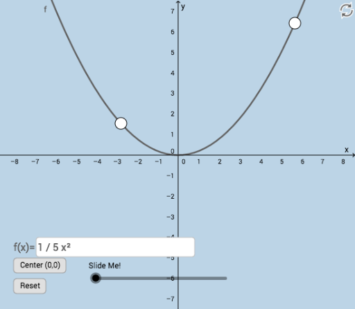
This example dynamically illustrates the Mean Value Theorem through geometric transformations, visually demonstrating the equality between the average rate of change of a function over an interval and the slope of a tangent at a point. Key math concepts include the Mean Value Theorem, derivatives, and geometric transformations. It utilizes commands/objects like Line, Slope, Intersect, Tangent, Circle, Dilate, Segment, Polygon, Angle, Ray, Vector, Translate, and Textfield in GeoGebra. Suitable for high school students and educators to grasp the geometric interpretation of the theorem and enhance intuitive understanding.
GeoGebra Commands & Parameters
Line(A, B) → gSlope(g) → mIntersect(n, h, 1) → CIntersect(i, j) → DTangent(D, f) → kIntersect(f, k) → ECircle(A, d) → eIntersect(e, l, 2) → FIntersect(g, p) → GIntersect(g, q) → HIntersect(g, r) → IDilate(A, If[0 < o ≤ 1, 1 - o, 0], B) → A'Segment(A, A') → f_1Intersect(k, s) → JIntersect(k, t) → KDilate(G, If[1 < o ≤ 2, 2 - o, 0], F) → G'Segment(G, G') → g_1Dilate(F, If[2 < o ≤ 3, 3 - o, 0], A) → F'Segment(F, F') → h_1Polygon(A, G, F) → poly1, f_2, a_1, g_2Angle(G, F, A) → αDilate(E, If[4 < o ≤ 5, 5 - o, 0], J) → E'Dilate(E, If[4 < o ≤ 5, 5 - o, 0], K) → E'_1Segment(E, E'_1) → i_1Segment(E, E') → j_1Intersect(k, q) → LIntersect(k, r) → MRay(K, M) → k_1Ray(J, L) → l_1Ray(B, I) → m_1Ray(A, H) → n_1Dilate(A, If[5 < o ≤ 6, 6 - o, 0], E) → A'_1Vector(A, A'_1) → uTranslate(A, u) → A'_2Translate(G, u) → G'_1Translate(F, u) → F'_1Polygon(A'_2, G'_1, F'_1) → poly1', f'_1, a'_2, g'_1Translate(F, u) → F'_2Translate(F', u) → F''Segment(F'_2, F'') → p_1Translate(G, u) → G'_2Translate(G', u) → G''Segment(G'_2, G'') → q_1Angle(G'_2, F'_2, A'_2) → βSegment(A'_2, G'_2) → r_1Textfield(f) → InputBox1
AI Drawing Prompt Reference
Illustrate the Mean Value Theorem by showing the average rate of change of a function over an interval equals the slope of a tangent at a point. Draw the function curve and interval, calculate the average rate, and plot the corresponding line. Find the intersection point of this line with the function. Then, draw the tangent at the point and locate the tangent point. Use geometric transformations like dilation, translation, and rotation with circles and segments to demonstrate relationships, highlighting key areas with polygons and angle measurements.
The prompt above was compiled from the original drawing commands and is for reference only.