
Maximum Likelihood Estimators
Loading the math board and drawing, please wait…
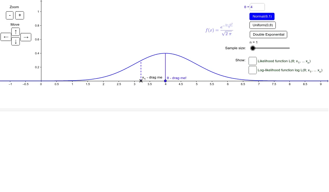
This example demonstrates the maximum likelihood estimator and log-likelihood function for various statistical models, covering core concepts like maximum likelihood estimation and probability density functions. It is constructed using GeoGebra commands like Point, Segment, Textfield, Uniform, Ray, and involves probability density functions such as doubleExpPDF, uniformPDF, and normPDF. Suitable for high school students and statistics learners.
GeoGebra Commands & Parameters
Point(xAxis) → x10Point(xAxis) → x9Point(xAxis) → x8Point(xAxis) → x7Point(xAxis) → x6Point(xAxis) → x5Point(xAxis) → x4Point(xAxis) → x3Point(xAxis) → x2Point(xAxis) → x1Point(xAxis) → thetaPointSegment(x1, (x(x1), f(x(x1)))) → linex1Textfield(thetaDummy) → thetaInputSegment(x2, (x(x2), f(x(x2)))) → linex2Segment(x3, (x(x3), f(x(x3)))) → linex3Segment(x4, (x(x4), f(x(x4)))) → linex4Segment(x5, (x(x5), f(x(x5)))) → line5Segment(x6, (x(x6), f(x(x6)))) → line6Segment(x7, (x(x7), f(x(x7)))) → line7Segment(x8, (x(x8), f(x(x8)))) → line8Segment(x9, (x(x9), f(x(x9)))) → line9Segment(x10, (x(x10), f(x(x10)))) → line10Segment(thetaPoint, (x(thetaPoint), f(x(thetaPoint)))) → linethetaUniform(0, thetaDummy, x) → funifRay(thetahatPoint, (x(thetahatPoint), -1)) → thetahatray1Point({theta, L(theta)}) → LthetaRay(thetaPoint, (x(thetaPoint), -1)) → thetaray1Point({theta, LogL(theta)}) → LogLthetaRay(LogLtheta, (x(thetaPoint), 1)) → thetaraylogPoint({x(thetahatPoint), LogL(x(thetahatPoint))}) → LogLthetahatPoint({x(thetahatPoint), L(x(thetahatPoint))}) → LthetahatRay(Ltheta, (x(thetaPoint), 1)) → thetaray2Ray(LogLthetahat, (x(thetahatPoint), yscale)) → thetahatraylogRay((x(thetahatPoint), L(x(thetahatPoint))), (x(thetahatPoint), yscale)) → thetahatray2
AI Drawing Prompt Reference
Draw a graph of maximum likelihood estimation for statistical models, including 10 points on the x-axis with corresponding lines representing probability density functions for double exponential, uniform, and normal distributions. Include a text input for parameter θ and its estimate θ̂. Show the likelihood and log-likelihood functions for θ̂, including the likelihood line for θ̂, the log-likelihood line for θ̂, the intersection point of the likelihood and log-likelihood functions for θ̂, and the slope lines for the likelihood and log-likelihood functions of θ̂.
The prompt above was compiled from the original drawing commands and is for reference only.