
Mathematical Principles of Earth's Sunrise and Sunset Phenomena
Loading the math board and drawing, please wait…
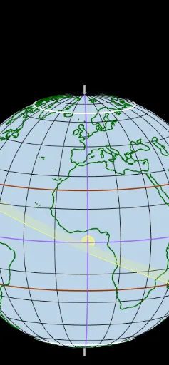
This example demonstrates the mathematical principles behind Earth's sunrise and sunset phenomena, involving concepts such as coordinate geometry, trigonometric functions, and analytic geometry. The construction uses GeoGebra commands like coordinate systems, rotation, circles, and lines to create relevant graphs. Suitable for high school students or college freshmen to explore the intersection of astronomy and mathematics.
GeoGebra Commands & Parameters
If(dia > 287, dia - 287, dia + 78) → diasIf(dia < 13, dia + 19, If[dia < 43, dia - 12, If[dia < 74, dia - 42, If[dia < 104, dia - 73, If[dia < 135, dia - 103, If[dia < 166, dia - 134, If[dia < 196, dia - 165, If[dia < 227, dia - 195, If[dia < 257, dia - 226, If[dia < 288, dia - 256, If[dia < 319, dia - 287, If[dia < 347, dia - 318, dia - 346]]]]]]]]]]]) → diaMesIf(dia < 13 ∨ dia > 346, 3, If[dia < 43, 4, If[dia < 74, 5, If[dia < 104, 6, If[dia < 135, 7, If[dia < 166, 8, If[dia < 196, 9, If[dia < 227, 10, If[dia < 257, 11, If[dia < 288, 12, If[dia < 319, 1, 2]]]]]]]]]]) → mesIf(mes < 3, mes + 12, mes) → mes1Rotate((0, 5, 0), oblicuidad, (0, 0, 0), xAxis) → EcOrthogonalLine((0, 0, 0), Plane[(0, 0, 0), (5, 0, 0), Ec]) → lCircle(l, (7, 0, 0)) → eclipticaSegment(PS + (0.075 * PS), PN + (0.075 * PN)) → ejeCircle((0, 0, 0), 5, eje) → ecuadorRay((0, 0, 0), A) → laserASphere((0, 0, 0), (0.999 * 5)) → tierraVector((1; (-rot) + 180°; (-inclinacion))) → dirCircle((5; 0; (-anguloPolar)), (5; 90°; (-anguloPolar)), (5; 180°; (-anguloPolar))) → antarticoCircle((5; 0; anguloPolar), (5; 90°; anguloPolar), (5; 180°; anguloPolar)) → articoCircle((5; 0; oblicuidad), (5; 90°; oblicuidad), (5; 180°; oblicuidad)) → cancerCircle((5; 0; (-oblicuidad)), (5; 90°; (-oblicuidad)), (5; 180°; (-oblicuidad))) → capricornioSequence(Circle[(5; 0; (15° * k)), (5; 90°; (15° * k)), (5; 180°; (15° * k))], k, 1, 5) → paralelosNSequence(Circle[(5; 0; (-15° * k)), (5; 90°; (-15° * k)), (5; 180°; (-15° * k))], k, 1, 5) → paralelosSCircle(SolDirecto, 0.25, Vector[SolDirecto, Sol]) → solDirectoElement(meses, mes) → mesTextoVector(SolDirecto) → vUnitVector(Vector[EQ]) → mIf(tt4 < 10, ("0" * tt4), ("" * tt4)) → t4Element(tiempo, 2) → segundosCircle(PN, (5; f; 0), PS) → greenwichCircumcircleArc(PN, (5; f + lonA; 0), PS) → meridianoAIf(tt3 < 10, ("0" * tt3), ("" * tt3)) → t3Line(Sol, laserA) → hOrthogonalPlane((0, 0, 0), laserA) → planoHorizonteAIntersect(h, planoHorizonteA) → COrthogonalLine(PN, planoHorizonteA) → jIntersect(j, planoHorizonteA) → PN'Vector(PN') → vectorPNVector(C) → vectorSolSegment(Sol, C) → pSegment(PN, PN') → qAngle(C, (0, 0, 0), Sol) → elevacion0Segment((0, 0, 0), Sol) → iSurface((((5.03 * cos(u)) * sin(v)) * x1) + (((5.03 * sin(u)) * sin(v)) * x3) - (((5.03 * cos(v)) * y(m)) * sin(β)), (((5.03 * cos(u)) * sin(v)) * x3) + (((5.03 * sin(u)) * sin(v)) * x2) + (((5.03 * cos(v)) * x(m)) * sin(β)), ((((5.03 * cos(u)) * sin(v)) * y(m)) * sin(β)) - ((((5.03 * sin(u)) * sin(v)) * x(m)) * sin(β)) + ((5.03 * cos(v)) * cos(β)), u, 0, π, v, π / 2, (3 * π / 2)) → aCircle((0, 0, z(Sol)), Sol, Vector[(0, 0, 1)]) → circuloAparenteSolIntersect(planoHorizonteA, circuloAparenteSol) → Sunset, SunriseCircumcircleArc(Sunset, Sol, Sunrise) → trayectoriaAparenteSolCircumcircleArc(PN1, (((2 * (hora - UT ≤ 12)) - 1) * M), Sol1) → arcoAcimutCircle((0, 0, 0), 7, laserA) → horizonteASequence(DJ0 - 2451545 + k - If[k > 287, 365, 0], k, 1, 365) → secNSequence(Mod[280.46 + (0.98565 * Element[secN, k]), 360]°, k, 1, 365) → secLSequence(Mod[357.528° + (0.9856° * Element[secN, k]), 360]°, k, 1, 365) → secGSequence(Element[secL, k] + (1.915° * sin(Element[secG, k])) + (0.02° * sin((2 * Element[secG, k]))), k, 1, 365) → secLandaSequence(asin((sin(oblicuidad) * sin(Element[secLanda, k]))), k, 1, 365) → secDeclinacionSequence(atan2((cos(oblicuidad) * sin(Element[secLanda, k])), cos(Element[secLanda, k])), k, 1, 365) → secARSequence(((2 * π / 365) * (If[k > 287, k - 287, k + 78] - 1 + (hora - UT - 12) / 24)), k, 1, 365) → secTiempo1Sequence(((229.18 * (0.00075 + (0.00187 * cos(Element[secTiempo1, k])) - (0.03208 * sin(Element[secTiempo1, k])) - (0.01462 * cos((2 * Element[secTiempo1, k]))) - (0.04085 * sin((2 * Element[secTiempo1, k])))) / 4) * π / 180), k, 1, 365) → secTiempoSequence((7; AR + Element[secTiempo, k]; Element[secDeclinacion, k]), k, 1, 365) → secAnalemaIf(lonA1 < -180°, lonA1 + 180°, If[lonA1 > 180°, lonA1 - 360°, lonA1]) → lonA2Sequence(Circle[PN, (5; f + (15° * k); 0), PS], k, 1, 11) → meridianosCircumcircleSector(Aries, (7; (AR + ecTiempo) / 2; 0), Sol2) → arcoARCircumcircleSector(Sol2, (7; AR + ecTiempo; declinacion / 2), Sol) → arcoDeclinacion
AI Drawing Prompt Reference
Draw a 3D sphere model of the Earth with the equator, poles, and lines of latitude and longitude. Include points for sunrise and sunset, the sun's position, the path of the sun, and arcs of the Earth's surface and visible face. The diagram illustrates the relationship between Earth's rotation and solar illumination, combining astronomy and mathematics.
The prompt above was compiled from the original drawing commands and is for reference only.