Mapping Diagrams for Visualizing Polynomial Roots

Loading the math board and drawing, please wait…

2018-04-08 18:37

In collections Mapping Diagrams to Visualize Complex Analysis

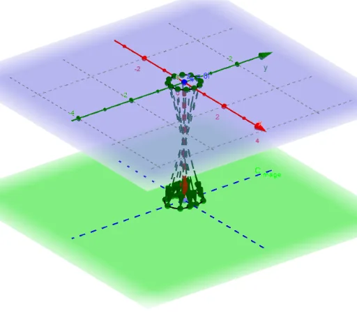
This example demonstrates how mapping diagrams can be used to visualize the roots of polynomials. It involves core mathematical concepts such as polynomial functions, complex roots, and mapping relationships. GeoGebra commands like Element, ComplexRoot, Sequence, Zip, Vector, CurveCartesian, PointIn, Intersect, Circle, Center, Point, Locus, and Radius are utilized to construct the diagram. It is suitable for high school and above students to understand the properties and visualization of polynomial roots.

GeoGebra Commands & Parameters

Element(fnl, deg_1 - 2) → fn
ComplexRoot(fn) → r_1, r_2, r_3, r_4, r_5, r_6
Sequence((δ * (cos(t) + (sin(t) * ί))) + real(z_#) + (imaginary(z_#) * ί), t, -3.14159, pi, (2 * pi / m)) → z_*
Zip(fn(z), z, z_*) → fz_*
Sequence((x(Element[fz_*, k]), y(Element[fz_*, k]), height_{image}), k, 1, m) → fpoint_*
Vector(z_#, f_{(z#).}) → w
CurveCartesian(t, 0, height_{image}, t, -5, 5) → Xh
CurveCartesian(0, t, height_{image}, t, -5, 5) → Yh
PointIn(C_{image}) → L
Sequence(Vector[Element[z_*, j], Element[fpoint_*, j]], j, 1, m) → fvec_*
Intersect(fn, xAxis) → A, B, C, D
Zip(Vector[(x(z), y(z), 0), (0, 0, height_{image})], z, roots) → rootsvec
Circle(r_3, r_2, r_1) → c
Center(c) → O_r
Point(circle) → P_C
Locus(F_D, P_C) → f_{circ}
Radius(c) → δ_r

AI Drawing Prompt Reference

Create a mapping diagram to visualize polynomial roots, highlighting core mathematical concepts. Start by plotting the polynomial function and marking its complex roots in the complex plane. Then, draw arrows from each root to the function's image to show the mapping relationships. Add coordinate axes and grids, highlight key points and loci, and use a circle to emphasize specific roots, completing the visualization.

The prompt above was compiled from the original drawing commands and is for reference only.