
Mapping Diagram for Complex Function Limits
Loading the math board and drawing, please wait…
In collections
Mapping Diagrams to Visualize Complex Analysis
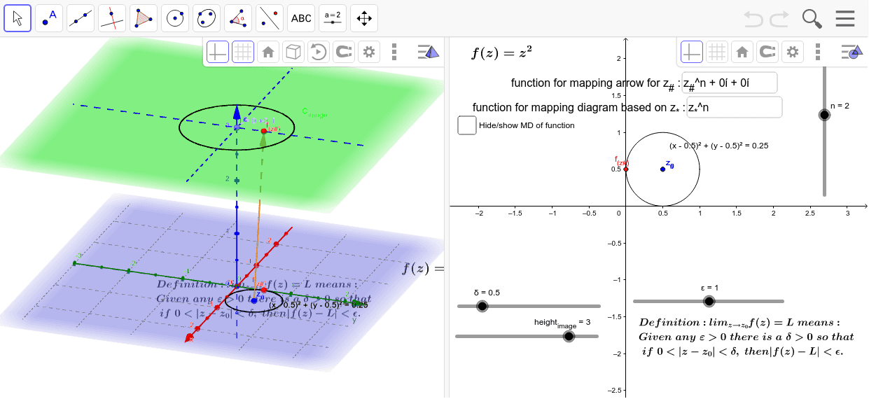
This example demonstrates the mapping diagram for limits of complex functions. It involves core mathematical concepts such as complex numbers, limits, and function mapping. The construction uses GeoGebra commands like Sequence, CurveCartesian, Textfield, Vector, PointIn, and Circle, with objects including z_0, δ, z_*, e, z_#, n, b, a, height_{image}, C_{image}, fz_*, C_{domain}, f_{(z#)}, f_{(z#).}, fpoint_*, fvec_*, d, inputBox1, w, inputBox2, Xh, Yh, inputBox3, text1, text2, L, ε, f, c, text3. It is suitable for high school and above students to understand the geometric meaning of complex function limits.
GeoGebra Commands & Parameters
Sequence((δ * (cos(t) + (sin(t) * ί))) + x(z_0) + (y(z_0) * ί), t, -3.14159, 3.141592653589793, 0.5236) → z_*Sequence((x(Element[fz_*, k]), y(Element[fz_*, k]), height_{image}), k, 1, 12) → fpoint_*Sequence(Vector[Element[z_*, j], Element[fpoint_*, j]], j, 1, 12) → fvec_*CurveCartesian((δ * cos(t)), (δ * sin(t)), height_{image}, t, 0, 6.283185307179586) → dTextfield(fz_*) → inputBox1Vector(z_#, f_{(z#).}) → wTextfield(f_{(z#)}) → inputBox2CurveCartesian(t, 0, height_{image}, t, -5, 5) → XhCurveCartesian(0, t, height_{image}, t, -5, 5) → YhTextfield(z_*) → inputBox3PointIn(C_{image}) → LCircle(L, ε, Vector[(0, 0, 1)]) → f
AI Drawing Prompt Reference
Draw a mapping diagram for complex function limits, showing a central point z_0 with a surrounding δ range, vectors from z_0 to mapped points f(z*), and curves for mapping paths, including input boxes and text labels, with a circle representing ε neighborhoods to illustrate the geometric meaning of complex function limits.
The prompt above was compiled from the original drawing commands and is for reference only.