
Magnus Effect on Balloon Trajectory
Loading the math board and drawing, please wait…
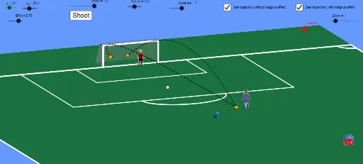
This example demonstrates how the Magnus effect influences the trajectory of a balloon. It involves core mathematical concepts such as vectors, function graphs, trigonometry, coordinate geometry, and probability & statistics. Key GeoGebra commands used in construction include Vector, OrthogonalLine, Translate, Segment, Mirror, Line, Intersect, Polygon, Midpoint, Point, Sequence, and CurveCartesian. It is suitable for high school and above students to explore the intersection of fluid dynamics and mathematics.
GeoGebra Commands & Parameters
Vector(B_1, Y) → vVector(B_1, X) → uVector(B_1, Z) → wOrthogonalLine(View3D, yAxis) → aOrthogonalLine(View3D, xAxis) → bTranslate(O, Vector[(8 * v)]) → OOSegment(O, OO) → dTranslate(O, u) → O'Mirror(O', O) → O''Segment(O'', O') → eLine(OO, e) → hLine(O'', d) → iLine(O', d) → jIntersect(i, h) → AIntersect(j, h) → BMirror(OO, A) → CMirror(OO, B) → DSegment(E, F) → lSegment(E, A) → mSegment(F, B) → nPolygon(C, D, H, G) → poly1, c_1, d_1, h_1, g_1Mirror(OO, C) → IMirror(OO, D) → JMirror(OO, I) → KMirror(OO, J) → LLine(L, j) → pLine(M, h) → qLine(K, i) → rIntersect(q, r) → NLine(P, h) → sMirror(L, P) → L'Intersect(s, r) → QLine(L', s) → a_1Intersect(a_1, r) → RPolygon(R, N, M, L') → poly2, r_1, n_1, m_1, l'Midpoint(Q, P) → S_1Polygon(R, K, L, L') → poly3, r_2, k_2, l_1, l'_1Line(O', O'') → b_1Line(V, h) → e_1Intersect(r_1, e_1) → TIntersect(m_1, e_1) → USegment(T, U) → f_1Point(f_1) → SVector(S, OO) → zSequence((x(S), y(S)) + (i / Distance * z) + (w * ((i * tan(α)) - ((0.5 * g / (((v_0 / 10)^(2) * cos(α)^(2)))) * i^(2)))), i, 0, Shoot, 0.1) → liste1Sequence((x(S), y(S)) + (i / Distance * z) + (w * ((i * tan(α)) - ((0.5 * g / (((v_0 / 10)^(2) * cos(α)^(2)))) * i^(2)))) + (u * ((i * tan(Effet)) - ((0.5 * g / (((v_0 / 10)^(2) * cos(Effet)^(2)))) * i^(2)))), i, 0, Shoot, 0.1) → liste2Midpoint(h_1) → WCurveCartesian(x(K + ((0.5 * cos(i)) * u) - ((0.5 * sin(i)) * v)), y(K + ((0.5 * cos(i)) * u) - ((0.5 * sin(i)) * v)), i, 0, 1.5707963267948966) → oCurveCartesian(x(L - ((0.5 * cos(i)) * u) - ((0.5 * sin(i)) * v)), y(L - ((0.5 * cos(i)) * u) - ((0.5 * sin(i)) * v)), i, 0, 1.5708) → i_1Line(I, i) → j_1Line(J, j) → p_1Line(A_1, k_2) → q_1Intersect(j_1, q_1) → C_1Intersect(p_1, q_1) → D_1Intersect(j_1, f_1) → E_1Segment(I, C_1) → s_1Segment(C_1, D_1) → t_1Segment(D_1, J) → a_2Midpoint(W, A_1) → F_1CurveCartesian(x(A_1 + ((1.5 * cos(i)) * u) - (sin(i) * v)), y(A_1 + ((1.5 * cos(i)) * u) - (sin(i) * v)), i, 0, 3.141592653589793) → o_1CurveCartesian(x(S_1 + ((2.5 * cos(i)) * u) - ((2.5 * sin(i)) * v)), y(S_1 + ((2.5 * cos(i)) * u) - ((2.5 * sin(i)) * v)), i, 0, 6.28319) → u_1Segment(Q, P) → b_2Segment(F, K_1) → c_2Segment(H_1, E) → f_2Polygon(K_1, I_1, G_1, H_1) → poly4, k_3, i_2, g_2, h_2Intersect(h_2, k_3) → L_1Intersect(n, c_1) → M_1Polygon(L_1, F, M_1, I_1) → poly5, l_2, f_3, m_2, i_3Intersect(m, c_1) → O_1Polygon(H_1, E, O_1, G_1) → poly6, d_2, e_2, j_2, n_2CurveCartesian(x(S + (i / Distance * z) + (w * ((i * tan(α)) - ((0.5 * g / (((v_0 / 10)^(2) * cos(α)^(2)))) * i^(2))))), y(S + (i / Distance * z) + (w * ((i * tan(α)) - ((0.5 * g / (((v_0 / 10)^(2) * cos(α)^(2)))) * i^(2))))), i, 0, Shoot) → v_1CurveCartesian(x(S + (i / Distance * z) + (w * ((i * tan(α)) - ((0.5 * g / (((v_0 / 10)^(2) * cos(α)^(2)))) * i^(2)))) + (u * ((i * tan(Effet)) - ((0.5 * g / (((v_0 / 10)^(2) * cos(Effet)^(2)))) * i^(2))))), y(S + (i / Distance * z) + (w * ((i * tan(α)) - ((0.5 * g / (((v_0 / 10)^(2) * cos(α)^(2)))) * i^(2)))) + (u * ((i * tan(Effet)) - ((0.5 * g / (((v_0 / 10)^(2) * cos(Effet)^(2)))) * i^(2))))), i, 0, Shoot) → w_1
AI Drawing Prompt Reference
Draw a balloon trajectory diagram showing the Magnus effect. The diagram includes three main parts: the initial velocity vector of the balloon represented by three perpendicular vectors; the balloon's motion trajectory composed of multiple line segments and curves, including the ascending path and the curved path affected by the Magnus effect; and the rotation effect of the balloon achieved through mirroring and line segment connections. The overall presentation shows the balloon's motion trajectory and rotation effect, demonstrating the influence of the Magnus effect on the balloon's movement.
The prompt above was compiled from the original drawing commands and is for reference only.