
MacLaurin Polynomials and Mapping Diagrams
Loading the math board and drawing, please wait…
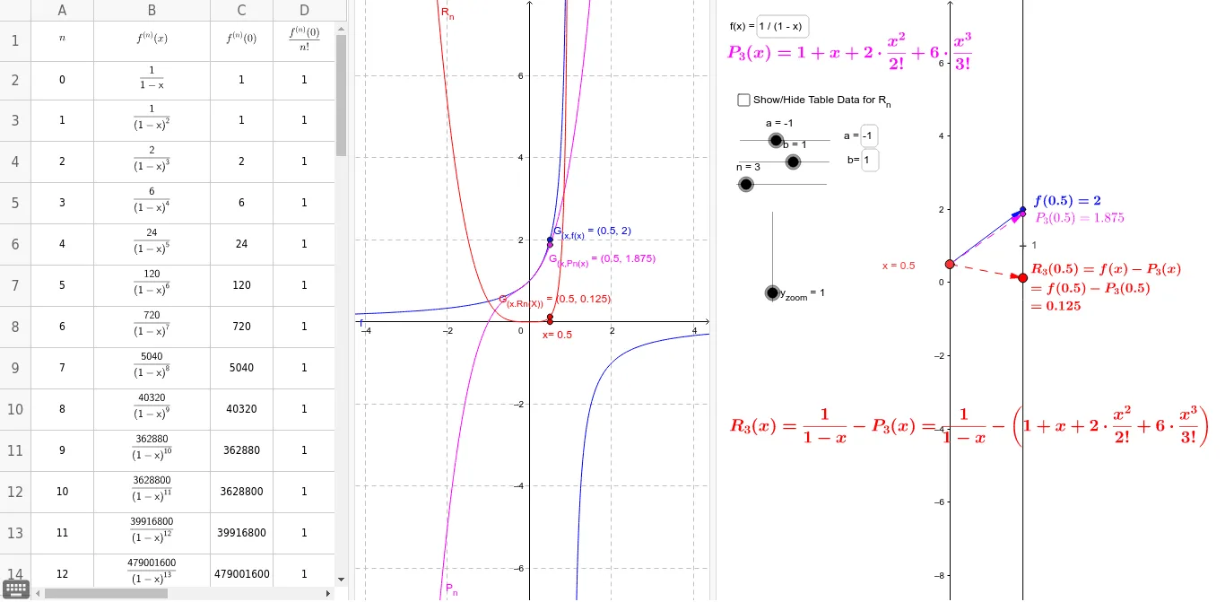
This example demonstrates MacLaurin polynomials and their corresponding mapping diagrams and graphs. It covers the concept of MacLaurin polynomials and how to use GeoGebra to draw the approximations of polynomial functions. By using commands like Point, TaylorSeries, Vector, Textfield, users can dynamically adjust the degree and center of the polynomial, observing the relationship between the polynomial and the original function. Suitable for high school mathematics education and learning.
GeoGebra Commands & Parameters
Point(yAxis) → P_xTaylorSeries(f, 0, n) → P_nVector(P_x, B) → uTextfield(f) → inputBox1Textfield(f) → inputBox2Textfield(a) → inputBox3Textfield(b) → inputBox4Sequence((0, k), k, a, b, Δx) → SourcePtsMDSegment((0, a), (0, b)) → cVector(P_x, F_x) → vVector(P_x, P_1) → wSequence((k, R_n(k)), k, a, b, Δx) → GraphptsSequence(Vector[(0, k), (2, (y_{zoom} * R_n(k)))], k, a, b, Δx) → MDSequence((2, (y_{zoom} * R_n(k))), k, a, b, Δx) → TargPts_1Derivative(f, A3) → B3Derivative(f, A4) → B4Derivative(f, A5) → B5Derivative(f, A6) → B6Derivative(f, A7) → B7Derivative(f, A8) → B8Derivative(f, A9) → B9Derivative(f, A10) → B10Derivative(f, A11) → B11Derivative(f, A12) → B12Derivative(f, A13) → B13Derivative(f, A14) → B14Derivative(f, A15) → B15Derivative(f, A16) → B16Derivative(f, A17) → B17Derivative(f, A18) → B18