
Lotka-Volterra System with Physical Space
Loading the math board and drawing, please wait…
In collections
SCIE1000
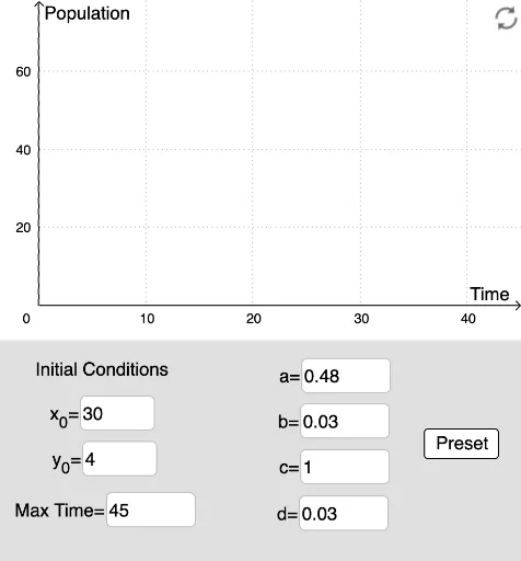
① This GeoGebra example demonstrates a Lotka-Volterra predator-prey model with a physical space, numerically solving the ODE system and visualizing the movement and population changes of prey and predators in a 2D plane. ② Core mathematical concepts include: predator-prey ecological modeling (Lotka-Volterra equations), numerical solution of ODE systems (NSolveODE), parameter sensitivity, phase-space trajectories, and population equilibrium. ③ Construction highlights: uses Polygon and Sequence to create background grids or regions, NSolveODE for solving differential equations, Textfield and InputBox for parameter input (a, b, c, d, timeMax, speedTime, etc.), Ray and Length for direction and distance display, buttons (button1-6) for animation, reset, or parameter control, objects like PredPosition and PreyPosition track positions, totalPrey and totalPred count totals, and pic1/pic2 may serve as background images or icons. ④ Suitable for high school to university courses in ecology, differential equations, or mathematical modeling, providing intuitive insight into population dynamics, phase portraits, and the impact of parameter changes on system stability.
GeoGebra Commands & Parameters
Polygon((200.185, -9), (-150, -9), 4) → poly1Polygon((20, -0.2), (-15, -0.2), 4) → poly2Sequence((RandomUniform[0, 10], RandomUniform[0, 10]), i, 1, 550) → PredPositionSequence((RandomUniform[0, 10], RandomUniform[0, 10]), i, 1, 550) → PreyPositionNSolveODE({y1', y2'}, -0.001, {ax, ay}, time) → num_1, num_2Length(num_1) → lenTextfield(ax) → InputBox1Textfield(ay) → InputBox2Textfield(a) → InputBox3Textfield(b) → InputBox4Textfield(c) → InputBox5Textfield(d) → InputBox6Sequence(Vector[(0, 0), Element[PredPosition, i]], i, 1, totalPred) → L_1Sequence(Vector[(0, 0), Element[PreyPosition, i]], i, 1, totalPrey) → L_2Sequence(Translate[pic1, Vector[Element[L_1, i]]], i, 1, totalPred) → L_3Sequence(Translate[pic2, Vector[Element[L_2, i]]], i, 1, totalPrey) → L_4Ray((time, 0), (time, x(B'))) → fTextfield(timeMax) → timeImput
AI Drawing Prompt Reference
Visualize predator-prey dynamics in a 2D plane using polygons for background grids, numerically solve differential equations to show trajectories, input parameters via sliders and text fields, use rays and lengths for direction and distance, control animations and resets with buttons, track positions of predators and prey, count totals, and incorporate images as backgrounds.
The prompt above was compiled from the original drawing commands and is for reference only.