Logistic Growth Model Interactive Demo

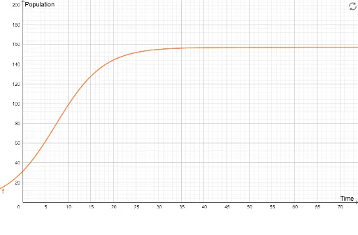
This GeoGebra example visually demonstrates the logistic growth model, illustrating how a population or quantity approaches a carrying capacity in an S-shaped curve over time. It focuses on the logistic differential equation dP/dt = rP(1-P/K), highlighting the roles of carrying capacity K, initial population P0, and growth rate r. The construction uses objects K, P0, r, and f, where K, P0, and r are likely adjustable sliders, and f represents the logistic function. Users can manipulate parameters to observe changes in the curve's steepness, inflection point, and asymptote. This is ideal for teaching differential equations, mathematical modeling, and population dynamics in high school or undergraduate courses, supporting interactive exploration of equilibrium solutions and parameter sensitivity.