
Lotka-Volterra System Model
Loading the math board and drawing, please wait…
In collections
UQ-Applied Mathematical Analysis
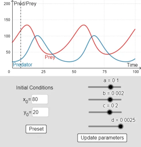
This example demonstrates the predator-prey dynamic system on a phase plane; involves core math concepts like differential equations, vector fields, parametric equations, and numerical solutions; constructed using GeoGebra commands/objects such as NSolveODE, SlopeField, Ray, Segment, Textfield, Polygon; suitable for high school students and educators to understand ecological mathematical models and calculus applications.
GeoGebra Commands & Parameters
NSolveODE({y1', y2'}, 0, {ax, ay}, 100) → num_1, num_2Length(num_1) → lenSlopeField((((d * x) * y) - (c * y)) / ((a * x) - ((b * x) * y)), 20, 0.5, 0, 0, 150, 150) → slopFRay(((ct * 100), 0), ((ct * 100), x(B))) → fSegment(C, B) → gSegment(B, D) → hTextfield(ax) → InputBox1Textfield(ay) → InputBox2Polygon((150, -25), (-150, -25), 4) → poly1
AI Drawing Prompt Reference
Draw a phase plane for a predator-prey dynamic system on a coordinate plane, showing numerical solutions of differential equations and a vector field, with rays and segments connecting key points, labeled parameters, and a quadrilateral framing the area, suitable for high school students and educators to understand ecological mathematical models and calculus applications.
The prompt above was compiled from the original drawing commands and is for reference only.