
Lotka-Volterra Model
Loading the math board and drawing, please wait…
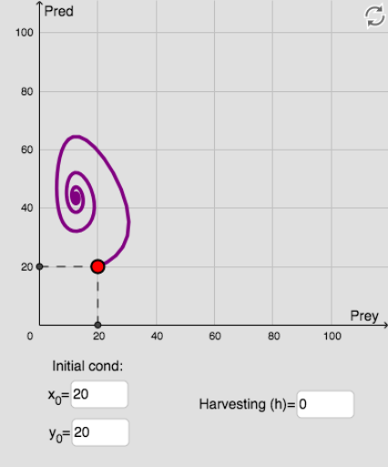
This example demonstrates the periodic population dynamics of predator-prey systems through graphical representations. Core math concepts include differential equations, function graphing, and continuity. Construction highlights involve commands like SolveODE, Length, First, Sequence, Element, Distance, Textfield, Ray, Text, NSolveODE, Point, Last, If, Segment, Polygon, Centroid in GeoGebra. Suitable for high school students and users interested in ecological mathematical models.
GeoGebra Commands & Parameters
SolveODE(g, f, x(A), y(A), time, step) → numericalIntegral1Length(numericalIntegral1) → len01First(numericalIntegral1, len01) → list1Sequence((floor((step * i)), x(Element[list1, i])), i, 1, len01) → listpreyElement(listprey, explore) → preyPointSequence((floor((step * i)), y(Element[list1, i])), i, 1, len01) → listpredatorElement(listpredator, explore) → predPointElement(list1, position) → BDistance(B, P2) → CondTextfield(x_0) → InputBox1Textfield(y_0) → InputBox2Textfield(h) → InputBox3Ray(timePoint, predPoint) → iText(("Pred=" * y(predPoint))) → textpreyText(("Prey=" * y(preyPoint))) → textpredNSolveODE({f1, g1}, 0, {x_0, y_0}, time) → numericalIntegral2, numericalIntegral2_2Point(numericalIntegral1) → CLast(listpredator) → LastpredatorElement(Lastpredator, 1) → MMIf(MM ≟ MM, MM, (1 / 2, 1 / 2)) → MMMSegment(D, C') → kSegment(E, C') → jPolygon(F, G, 5) → poly1, l, m, n, p, q, H, I, JCentroid(poly1) → K