Long Term Behaviour 2: Visualizing Differential Equation Solutions

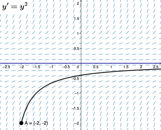
This GeoGebra example demonstrates the long-term behavior of solutions to a first-order differential equation using a slope field and numerical solving. It visualizes how solution curves evolve over time, highlighting concepts such as direction fields, initial value problems, and asymptotic stability. The construction employs the SlopeField command to draw the direction field, SolveODE to compute numerical solutions, and a slider (h) to adjust step size, with a button (button1) to animate. Objects like A, F, Sol1, and text1 support dynamic exploration of different initial conditions. Suitable for high school or college calculus and differential equations courses, it helps students understand solution trends, equilibrium points, and the impact of numerical accuracy on long-term predictions.