Logistic Growth with Extinction Threshold

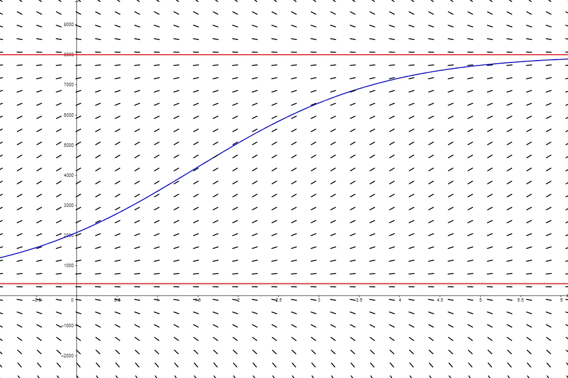
This GeoGebra example demonstrates the solution curves and slope field of a logistic growth model that includes an extinction threshold. The core mathematical concepts involve first-order ordinary differential equations, logistic growth dynamics, equilibrium points and stability, slope fields (direction fields), and initial value problems. The construction uses the SlopeField command to generate the direction field and SolveODE to numerically solve the differential equation. Sliders m, M, and k control the growth rate, carrying capacity, and extinction threshold, while P0 sets the initial population. The objects A and oplossing2 display particular solution curves for chosen initial conditions, with g and h as auxiliary functions and tekst1/tekst2 providing dynamic labels. This resource is suitable for high school to university-level mathematics instruction, helping students visualize population dynamics, interpret differential equations graphically, and explore ecological modeling concepts.