
Logarithmic Functions Graphing and Comparison
Loading the math board and drawing, please wait…
In collections
CCGPS AA Unit 4 Lesson 2
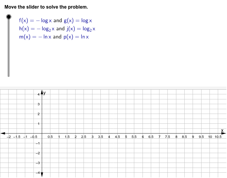
This example demonstrates graphing and comparing three pairs of logarithmic functions. It involves core math concepts like logarithmic function properties, graph translations, and asymptotes. GeoGebra commands and objects such as Sequence, LaTeX, TableText, Ray, and Text are used in construction. Suitable for high school mathematics teaching, helping students understand function graph transformations and property analysis.
GeoGebra Commands & Parameters
Sequence(x = a, a, -7, -4, 0.5) → list1LaTeX("\textcolor{#000099}{f(x)=-\log x}\text{ and }\textcolor{#000099}{g(x)=\log x}") → pair1LaTeX("\textcolor{#000099}{h(x)=-\log_{2} {x}}\text{ and }\textcolor{#000099}{j(x)=\log_{2} {x}}") → pair2LaTeX("\text{Three pairs of logarithmic functions are provided. Graph each pair on one coordinate}\cr\text{plane. Then, use the graphs to identify and compare the asymptotes, intercepts,}\cr \text{domains, and ranges for each pair, as well as the shape and end behavior of each pair}\cr \text{of graphs.}") → problemtextLaTeX("\textcolor{#000099}{m(x)=-\ln x}\text{ and }\textcolor{#000099}{p(x)=\ln x}") → pair3TableText({{pair1}, {pair2}, {pair3}}, "l") → text1LaTeX("\text{Graph the first pair of functions on the same coordinate plane.}") → text2LaTeX("\textcolor{#FF0000}{f(x)=-\log x}") → ftextLaTeX("\textcolor{#006400}{g(x)=\log x}") → gtextLaTeX("\text{Compare the shapes and end behavior of the graphs.}") → text3LaTeX("\text{The line of reflection is the }\textcolor{#FF00FF}\text{x-axis}\text{.}") → text4LaTeX((((("\text{The shape and end behavior of the graph of }\textcolor{#FF0000}{" * ftext) * "}\text{ are inverted}\cr \text{from the shape and end behavior of the graph of }\textcolor{#006400}{") * gtext) * "}\text{. In}\cr \text{other words, the two graphs are reflections of each other.} ")) → text33LaTeX((((("\text{The graph of }\textcolor{#FF0000}{" * ftext) * "}\text{ decreases as }\textcolor{#000099}\text{x}\text{ approaches positive infinity.}\cr \text{The graph of }\textcolor{#006400}{") * gtext) * "}\text{ increases as }\textcolor{#000099}\text{x}\text{ approaches positive infinity.}")) → text5LaTeX("\text{Identify the two graphs’ asymptotes, intercepts, domains, and ranges.}") → text6LaTeX("\text{Since neither graph crosses the }\textcolor{#000099}\text{y-axis}\text{, both graphs have a vertical}\cr\text{asymptote at }\textcolor{#FF00FF}\text{x = 0}\text{.}") → text7LaTeX("\text{The graphs cross the }\textcolor{#000099}\text{x-axis}\text{ at the x-intercept }\textcolor{#000099}{\left(1, 0 \right)}\text{.}") → text8LaTeX("\text{Since the }\textcolor{#000099}{x-values}\text{ increase into positive infinity but never cross the}\cr\textcolor{#000099}{y-axis}\text{, this means they are never negative. Thus, we can determine the}\cr\text{domain of both graphs is }\textcolor{#000099}{x > 0}\text{.}") → text9Ray((0.1, 0), (1, 0)) → cLaTeX("\text{The range of both graphs is }{\textcolor{#000099}\text{all real numbers}\text{.}") → text10LaTeX("\text{Graph the second pair of functions together on a new coordinate plane.}") → text11LaTeX("\textcolor{#006400}{j(x)=\log_{2}{x}}") → jtextLaTeX("\textcolor{#FF0000}{h(x)=-\log_{2}{x}}") → htextLaTeX((((("\text{The graph of }\textcolor{#006400}{" * jtext) * "}\text{ and }\textcolor{#FF0000}{") * htext) * "}\text{ is shown.}")) → text111LaTeX("\text{Compare the shapes and end behavior of the second pair of graphs.}") → text12LaTeX((((("\text{The shape and end behavior of the graph of }{" * htext) * "}\text{ are inverted}\cr\text{from that of }{") * jtext) * "}\text{. In other words, each graph is a reflection of}\cr\text{the other over the }\textcolor{#FF00FF}\text{x-axis}\text{.}")) → text122LaTeX((((("\text{The graph of }{" * htext) * "}\text{ decreases as }\textcolor{#000099}\text{x}\text{ approaches positive infinity.}\cr \text{The graph of }{") * jtext) * "}\text{ increases as }\textcolor{#000099}\text{x}\text{ approaches positive infinity.}")) → text13LaTeX("\text{Identify the two graphs’ asymptotes, intercepts, domains, and ranges.}") → text14LaTeX("\text{There is a vertical asymptote at }{\textcolor{#FF00FF}\text{x = 0}\text{ for each graph.}") → text15LaTeX("\text{Both graphs cross the }\textcolor{#000099}\text{x-axis}\text{ at the x-intercept }\textcolor{#000099}{\left(1, 0\right)}\text{.}") → text16LaTeX("\text{The domain of both graphs is }\textcolor{#000099}\text{x > 0}\text{.}") → text17LaTeX("\text{Since the y-values are not limited, we can determine the range of each graph}\cr\text{is }\textcolor{#000099}\text{all real numbers}\text{.}") → text18LaTeX("\text{Graph the third pair of functions together on a new coordinate plane.}\cr \text{Compare the graphs’ shapes and end behavior.}") → text19LaTeX("\textcolor{#006400}{p(x)=\ln x}") → ptextLaTeX("\textcolor{#FF0000}{m(x)=-\ln x}") → mtextLaTeX((((("\text{The graph of }{" * ptext) * "}\text{ and }{") * mtext) * "}\text{ is shown.}")) → text20LaTeX((((("\text{The shape and end behavior of the graph of }{" * mtext) * "}\text{ are inverted}\cr \text{from that of }{") * ptext) * "}\text{; therefore, the graphs are reflections of one}\cr\text{another. The line of reflection is the }\textcolor{#FF00FF}\text{x-axis}\text{.}")) → text21LaTeX((((("\text{The graph of }{" * mtext) * "}\text{ decreases as }\textcolor{#000099}\text{x}\text{ approaches positive infinity.}\cr\text{The graph of }{") * ptext) * "}\text{ increases as }\textcolor{#000099}\text{x}\text{ approaches positive infinity.}")) → text22LaTeX((((("\text{Graph the given functions, }{" * ftext) * "}\text{ and }{") * gtext) * "}\text{, by hand or}\cr\text{using a graphing calculator. The result should resemble the following.}")) → textnew2LaTeX("\text{Use the graphs to identify the asymptotes, intercepts, domains, and}\cr \text{ranges of this third pair of functions.}") → text23LaTeX("\text{There is a vertical asymptote at }\textcolor{#FF00FF}\text{x = 0}\text{.}") → text24LaTeX("\text{The graphs cross the x-axis at the x-intercept }\textcolor{#000099}{\left(1, 0\right)}\text{.}") → text25LaTeX("\text{The domain of both graphs is }\textcolor{#000099}\text{x > 0}\text{.}") → text26LaTeX("\text{The range of both graphs is }\textcolor{#000099}\text{all real numbers}\text{.}") → text27LaTeX("\text{Summarize your findings.}") → text28LaTeX("\text{In summary, all three pairs of graphs have the same vertical asymptote}\cr\text{of }\textcolor{#FF00FF}\text{x = 0}\text{. In every case, the x-intercept is }\textcolor{#000099}{\left(1, 0\right)}\text{. The domain and range}\cr \text{for all three pairs are identical. The three pairs of functions}\cr\text{differ in the rate of increase or decrease as }\textcolor{#000099}\text{x}\text{ increases.}") → text29Text("Move the slider to solve the problem.") → text0
AI Drawing Prompt Reference
Graph three pairs of logarithmic functions and compare them. The first pair, f(x)=-logx and g(x)=logx, are symmetric about the x-axis, intersect at x=1, have vertical asymptotes at x=0, and domains/ranges of x>0 and all real numbers respectively. The second pair, h(x)=-log2x and j(x)=log2x, share the same properties. The third pair, m(x)=-lnx and p(x)=lnx, also share the same properties. All graphs increase or decrease on the positive x-axis and are mirror images of each other.
The prompt above was compiled from the original drawing commands and is for reference only.