Linear Transformations of Function Graphs

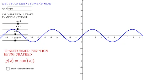
This example demonstrates how linear (affine) transformations modify a function’s graph, letting learners visually compare the original curve with the transformed one under different parameter choices. It focuses on key ideas such as function graphing, geometric interpretation of linear transformations, and how shifts and scalings of inputs/outputs affect the resulting curve. Construction-wise, the setup uses GeoGebra input and labeling tools: a Textfield-based interface to display parameters and equations; the original function object f; and multiple parameter inputs (a, h, k, b, c, d) to define the transformed function. The referenced InputBox1 and additional text objects (text1, text2, text3, text5) support interactive parameter entry and clear on-graph annotation. Suitable for secondary school through early college use, especially for instruction on transformation of graphs, function relationships, and interactive visualization in mathematics lessons.