
Linear Regression & Secant/Tangent Function Demo
Loading the math board and drawing, please wait…
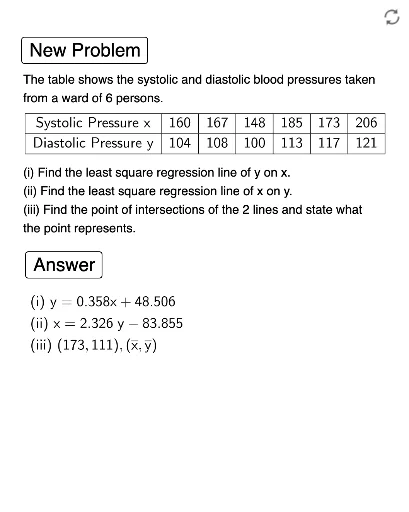
This example demonstrates the dynamic behavior of linear regression, secant lines, and tangent functions in a coordinate system. Key math concepts include linear regression, secant, tangent function, statistics, and ellipse. Construction highlights GeoGebra commands like Length, Sequence, FitLineY, Shuffle, TableText, and Join. Suitable for high school students and educators exploring data analysis and function properties.
GeoGebra Commands & Parameters
Length(lx) → nSequence((Element[lx, i], Element[ly, i]), i, 1, n) → l1FitLineY(l1) → fSequence(round(f(Element[lx, i]) + ((-1)^(Random[1, 2]) * Random[3, 6]), 0), i, 1, n) → ly1Sequence((Element[lx, i], Element[ly1, i]), i, 1, n) → l3Shuffle(l3) → l4, {(160, 104), (167, 108), (148, 100), (185, 113), (173, 117), (206, 121)}Sequence((Element[ly1, i], Element[lx, i]), i, 1, n) → l2FitLineY(l2) → gTableText(lx, ly1, "c") → text1Join({{"Systolic Pressure x"}, Sequence[x(Element[l4, i]), i, 1, n]}) → l5Join({{"Diastolic Pressure y"}, Sequence[y(Element[l4, i]), i, 1, n]}) → l6TableText(l5, l6, "c|_") → text2FitLineY(l4) → f1Sequence((Element[l5, i], Element[l6, i]), i, 2, n) → l7