
Linear Regression Practice
Loading the math board and drawing, please wait…
In collections
AP Stats Exam Review
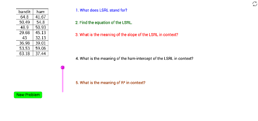
This example demonstrates how to perform linear regression analysis using GeoGebra. It involves plotting scatter plots, fitting lines, calculating the correlation coefficient (PMCC), and determining the coefficient of determination (RSquare). Key commands used include Random, Sequence, PMCC, FitLineY, RSquare, Intersect, Slope, RandomElement, and TableText. Suitable for high school or introductory college students learning data analysis and statistical modeling.
GeoGebra Commands & Parameters
Random(5, 9) → dataSequence(RandomNormal[50, 10] + a - a, a, 1, data) → explanatorySequence(RandomNormal[50, 10] + a - a, a, 1, data) → responsePMCC(explanatory, response) → rSequence((Element[explanatory, i], Element[response, i]), i, 1, data) → list1FitLineY(list1) → aRSquare(list1, a) → rrIntersect(a, yAxis) → ASlope(a) → mRandomElement(words2) → text5RandomElement(words) → text4TableText({Append[text4, explanatory], Append[text5, response]}, "|_vc") → text1
AI Drawing Prompt Reference
Create a linear regression analysis example with a scatter plot made of randomly generated points, a fitted line, and text displaying the correlation coefficient and coefficient of determination. First, plot the scatter points, then fit a line through them, label the intercept and slope of the line, and finally add text boxes next to the plot showing the correlation coefficient and coefficient of determination.
The prompt above was compiled from the original drawing commands and is for reference only.