
Linear Regression Demo
Loading the math board and drawing, please wait…
In collections
Pearson Maths A level Further Statistics 2
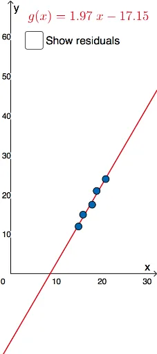
This example demonstrates the calculation and visualization process of linear regression, involving core concepts like linear regression equation, least squares method, slope, and standard deviation. GeoGebra commands used include Sequence, FitPoly, Slope, Vector, Min, and Max. Suitable for high school students and beginners in data analysis.
GeoGebra Commands & Parameters
Sequence(Segment[(-100, i), (100, i)], i, -50, 200, 1) → list1Sequence(Segment[(-100, i), (100, i)], i, -50, 200, 5) → list2Sequence(Segment[(i, -100), (i, 100)], i, -50, 50, 0.2) → list3Sequence(Segment[(i, -100), (i, 100)], i, -50, 50, 1) → list4FitPoly(list5, 1) → gSlope(g) → mVector(E, Ee) → uVector(Dd, D) → vVector(Cc, C) → wVector(Bb, B) → cVector(Aa, A) → dMin({x(A), x(B), x(C), x(D), x(E)}) → eMax({x(A), x(B), x(C), x(D), x(E)}) → fMin({y(A), y(B), y(C), y(D), y(E)}) → hMax({y(A), y(B), y(C), y(D), y(E)}) → i
AI Drawing Prompt Reference
Create a linear regression demonstration showing a grid of horizontal and vertical lines, a fitted line through data points using the least squares method, and the slope vector of the regression line. Mark the minimum and maximum x and y coordinates of all data points to illustrate the calculation and visualization process of linear regression.
The prompt above was compiled from the original drawing commands and is for reference only.