
Linear Regression & Correlation Exploration
Loading the math board and drawing, please wait…
In collections
AP Statistics
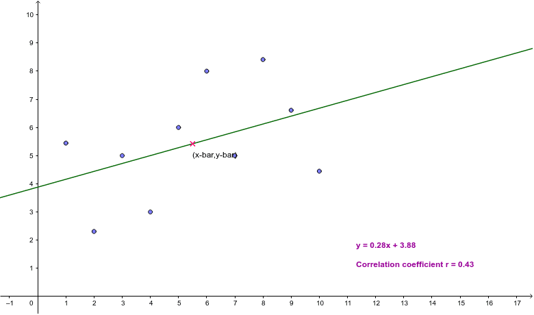
This example demonstrates linear modeling by manipulating (x, y) data points. It focuses on how the correlation coefficient r describes linearity. Key GeoGebra commands and objects used include Point, PMCC, FitLineY, and elements like A, B, C, r, corrcoef, f, centroid, fitting the model and visualizing statistical relationships, ideal for high school and introductory college statistics courses.
GeoGebra Commands & Parameters
Point(Line[(1, 0), (1, 2)]) → APoint(Line[(2, 0), (2, 2)]) → BPoint(Line[(3, 0), (3, 2)]) → CPoint(Line[(4, 0), (4, 2)]) → DPoint(Line[(5, 0), (5, 2)]) → EPoint(Line[(6, 0), (6, 2)]) → FPoint(Line[(7, 0), (7, 2)]) → GPoint(Line[(8, 0), (8, 2)]) → HPoint(Line[(9, 0), (9, 2)]) → IPoint(Line[(10, 0), (10, 2)]) → JPMCC({A, B, C, D, E, F, G, H, I, J}) → rFitLineY({A, B, C, D, E, F, G, H, I, J}) → f
AI Drawing Prompt Reference
Draw 10 points in a coordinate system where the points are evenly spaced along the x-axis with y-values ranging from 0 to 2. Calculate and display the correlation coefficient among these points. Then, fit a line to these points and show the equation of the line. The graph should clearly display the data points, the fitted line, and the correlation coefficient, suitable for statistics education.
The prompt above was compiled from the original drawing commands and is for reference only.