
Linear Regression by Jennifer Loveland
Loading the math board and drawing, please wait…
In collections
Statistical Applets
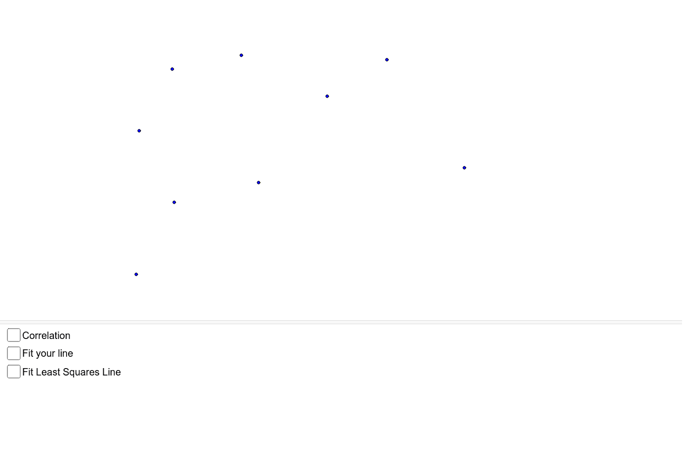
This example demonstrates how outliers affect correlation and the line of best fit. Attempt to create a line of best fit by minimizing SSE or MSE. Compare your line to … This example involves statistical characteristics. GeoGebra commands used include: Line, SumSquaredErrors, FitLineY, Distance, PMCC, Slope. Suitable for high school mathematics education.
GeoGebra Commands & Parameters
Line(J, K) → YOURSumSquaredErrors({A, B, C, D, E, F, G, H, I}, YOUR) → SSEYFitLineY({I, H, G, F, E, D, C, B, A}) → BESTSumSquaredErrors({A, B, C, D, E, F, G, H, I}, BEST) → SSEBDistance(B, E) → BEPMCC({A, B, C, D, E, F, G, H, I}) → rSlope(YOUR) → mYOURSlope(BEST) → mBEST
AI Drawing Prompt Reference
Draw a set of scatter points and plot the best-fit line obtained by minimizing the sum of squared errors, along with a regular line. Calculate and label the sum of squared errors for both lines, and display the distance between points and the point product correlation coefficient. Finally, label the slopes of both lines to show how the slope is adjusted by optimizing the error.
The prompt above was compiled from the original drawing commands and is for reference only.