
Linear Function Modeling of Automated Mower Time vs. Field Area
Loading the math board and drawing, please wait…
In collections
CCSS IP Math I Unit 4 Lesson 2
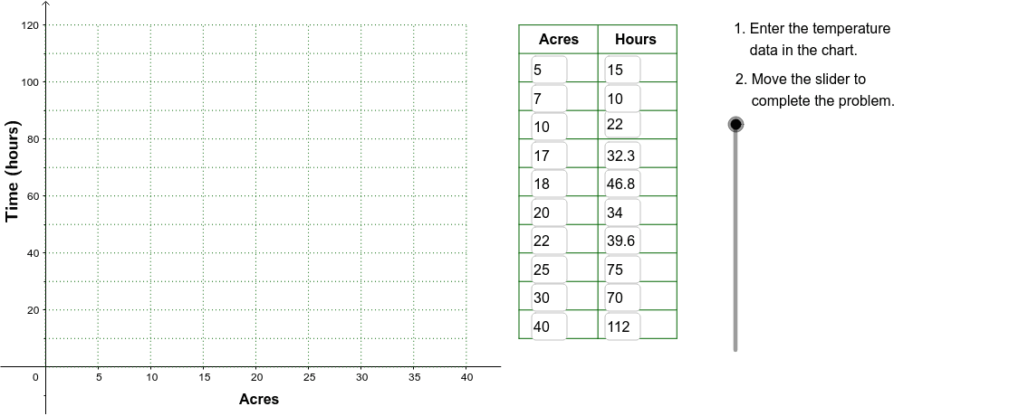
This GeoGebra example demonstrates how automated lawn mowers’ operating time varies linearly with field size across trials of different dimensions, using scatter plots and fitted lines to model real-world work efficiency. Core mathematical concepts include linear functions, function graphs, scatter plots, confidence intervals, natural numbers, arithmetic operations, ratios, and parallelogram area. The construction relies on GeoGebra commands and objects extracted from the summary: Corner generates field vertices, Polygon builds the field shape (poly1, corn1–corn4), Line draws the regression/fitted line, Sequence creates data points, Textfield and VerticalText provide labels, and the Slid object enables dynamic parameter adjustment; point objects A1–B9 support scatter data. Suitable for middle school and high school mathematics instruction, especially function modeling, statistics, and dynamic geometry exploration in classroom demonstrations or student inquiry activities.
GeoGebra Commands & Parameters
Corner(2) → Corn2Corner(3) → Corn3Polygon(Corn1, Corn2, Corn3, Corn4) → poly1, corn1, corn2, corn3, corn4Textfield(A2) → InA2Textfield(A3) → InA3Textfield(A4) → InA4Textfield(A5) → InA5Textfield(A6) → InA6Textfield(A7) → InA7Textfield(A8) → InA8Textfield(A9) → InA9Textfield(B9) → InB9Textfield(B8) → InB8Textfield(B7) → InB7Textfield(B6) → InB6Textfield(B5) → InB5Textfield(B4) → InB4Textfield(B3) → InB3Textfield(B2) → InB2Line(Pt1, Pt2) → FitLineSequence(Segment[(45, 10 + (10 * j)), (60, 10 + (10 * j))], j, 0, 11) → LnListSequence(Segment[(45 + (7.5 * j), 10), (45 + (7.5 * j), 120)], j, 0, 2) → LnList2Textfield(A10) → InA10Textfield(A11) → InA11Textfield(B10) → InB10Textfield(B11) → InB11VerticalText("\text{Time (hours)}") → DownLegendSequence(Segment[((5 * i), 0), ((5 * i), 120)], i, 0, 8) → GridxSequence(Segment[(0, (10 * i)), (40, (10 * i))], i, 0, 12) → Gridy
AI Drawing Prompt Reference
Create a parallelogram shape to represent the field, using four corner points to define its boundaries. Plot a series‑of scatter points that model the relationship between mowing time (in hours) and field area (in square meters), forming a data cloud. Draw a best‑fit straight line through these points to illustrate the linear regression. Add horizontal and vertical grid lines for easier reading. Label the vertical axis as “Time (hours)”. Include a slider to adjust the slope and intercept of the linear function, allowing dynamic exploration of how changes in the model affect the fit. The final diagram should clearly show the field, the data points, the regression line, grid, axis label, and interactive slider for classroom investigation.
The prompt above was compiled from the original drawing commands and is for reference only.