
Linear Equation Example
Loading the math board and drawing, please wait…
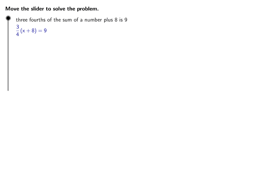
This example demonstrates converting a verbal statement into a mathematical equation. Key math concepts include linear equations. Construction highlights the use of If, LaTeX, Corner, FractionText, and TableText commands. Suitable for middle school math education.
GeoGebra Commands & Parameters
If(operation1 ≟ "sum", equals - simplen, equals + simplen) → newEqualsnLaTeX(steps) → counterLaTeX("\text{Use the buttons below to return to the original problem or}\cr\text{randomly generate a similar practice problem.}") → RandomizationTextCorner(1) → ACorner(3) → BLaTeX("\text{Apply the Distributive Property.}") → text1LaTeX("\text{Isolate the variable in the resulting equation.}") → text8FractionText(simplen) → simpleLaTeX((((((((((((((((((((((("\text{" * numWord) * " ") * denWord) * " of the ") * operation1) * " of a number ") * operation2) * " ") * add) * " is ") * equals) * "}\cr\textcolor{#000099}{\frac{") * num) * "}{") * denom) * "}\left(x") * operation3) * "") * add) * "\right)=") * equals) * "}")) → ProblemLaTeX((((("\text{The Distributive Property states that }\textcolor{#000099}{a(b " * operation3) * " c) = ab ") * operation3) * " ac}.")) → text2LaTeX((((((((((((((("\text{For }\textcolor{#000099}{\frac{" * num) * "}{") * denom) * "}\left(x") * operation3) * "") * add) * "\right)=") * equals) * "}\text{ each of the terms in parentheses needs to be multiplied by }\textcolor{#000099}{\frac{") * num) * "}{") * denom) * "}}.")) → text3LaTeX((("\text{Apply the " * operation4) * " Property of Equality.}")) → text10FractionText(newEqualsn) → newEqualsLaTeX((((((((("\text{In order to isolate the variable, the term }\textcolor{#000099}{\frac{" * num) * "}{") * denom) * "}x}\text{ must first be isolated. Look at the}\cr\text{operation being used on the term with }\textcolor{#000099}{\frac{") * num) * "}{") * denom) * "}x}\text{, and use the opposite operation to}\cr\text{isolate the term. }")) → text9FractionText(xvaln) → xvalLaTeX((((((((((((("\text{The value for }\textcolor{#000099}{x}\text{ in }\textcolor{#000099}{\frac{" * num) * "}{") * denom) * "}\left(x") * operation3) * "") * add) * "\right)=") * equals) * "}\text{ is }\textcolor{#000099}{") * xval) * "}.")) → text18LaTeX((((((("\text{By " * operation5) * " }\textcolor{#000099}{") * simple) * "}\text{ ") * operationPrep) * " both sides of the equation, both sides of the equation will}\cr\text{remain equal, but the term containing the variable }\textcolor{#000099}{x}\text{ will be isolated.}")) → text11TableText({{LaTeX[(((((((((("\textcolor{#000099}{\frac{" * num) * "}{") * denom) * "}\left(x") * operation3) * "") * add) * "\right)=") * equals) * "}")], LaTeX["\text{Original equation}"]}, {LaTeX[(((((((((((((("\textcolor{#000099}{\frac{" * num) * "}{") * denom) * "}x ") * operation3) * " \frac{") * num) * "}{") * denom) * "}(") * add) * ")=") * equals) * "}")], LaTeX["\text{Distribute.}"]}, {LaTeX[(((((((((("\textcolor{#000099}{\frac{" * num) * "}{") * denom) * "}x ") * operation3) * " ") * simple) * "=") * equals) * "}")], LaTeX["\text{Simplify.}"]}}, "l") → text6LaTeX((((((((((("\text{Once the Distributive Property is applied, the resulting equation is }\textcolor{#000099}{\frac{" * num) * "}{") * denom) * "}x ") * operation3) * " ") * simple) * "=") * equals) * ".}")) → text7TableText({{LaTeX[(((((((((("\textcolor{#000099}{\frac{" * num) * "}{") * denom) * "}x ") * operation3) * " ") * simple) * "=") * equals) * "}")], LaTeX["\text{Equation from the previous step}"]}, {LaTeX[(((((("\textcolor{#000099}{\frac{" * num) * "}{") * denom) * "}x =") * newEquals) * "}")], LaTeX[(((((("\text{" * operation6) * " }\textcolor{#000099}{") * simple) * "}\text{ ") * operationPrep) * " both sides of the equation.}")]}}, "l") → text13LaTeX((((("\text{In order to isolate }\textcolor{#000099}{x}\text{ from the term }\textcolor{#000099}{\frac{" * num) * "}{") * denom) * "}x}\text{, apply the Multiplication Property of Equality.}")) → text14TableText({{LaTeX[(((((("\textcolor{#000099}{\frac{" * num) * "}{") * denom) * "}x =") * newEquals) * "}")], LaTeX["\text{Equation from the previous step}"]}, {LaTeX[(("\textcolor{#000099}{x =" * xval) * "}")], LaTeX[(((("\text{Multiply both sides by the reciprocal, }\textcolor{#000099}{\frac{" * denom) * "}{") * num) * "}.}")]}}, "l") → text17TableText({{LaTeX[(((((((((("\textcolor{#000099}{\frac{" * num) * "}{") * denom) * "}\left(x") * operation3) * "") * add) * "\right)=") * equals) * "}")], LaTeX["\text{Original equation}"]}}, "l") → text4TableText({{LaTeX[(((((((((("\textcolor{#000099}{\frac{" * num) * "}{") * denom) * "}\left(x") * operation3) * "") * add) * "\right)=") * equals) * "}")], LaTeX["\text{Original equation}"]}, {LaTeX[(((((((((((((("\textcolor{#000099}{\frac{" * num) * "}{") * denom) * "}x ") * operation3) * " \frac{") * num) * "}{") * denom) * "}(") * add) * ")=") * equals) * "}")], LaTeX["\text{Distribute.}"]}}, "l") → text5TableText({{LaTeX[(((((((((("\textcolor{#000099}{\frac{" * num) * "}{") * denom) * "}x ") * operation3) * " ") * simple) * "=") * equals) * "}")], LaTeX["\text{Equation from the previous step}"]}}, "l") → text12TableText({{LaTeX[(((((("\textcolor{#000099}{\frac{" * num) * "}{") * denom) * "}x =") * newEquals) * "}")], LaTeX["\text{Equation from the previous step}"]}}, "l") → text16LaTeX("\text{Move the slider to solve the problem.}") → text0LaTeX((((((((("\text{By multiplying both sides of the equation by }\textcolor{#000099}{\frac{" * denom) * "}{") * num) * "}}\text{ (the reciprocal of }\textcolor{#000099}{\frac{") * num) * "}{") * denom) * "}}\text{), both sides}\cr\text{of the equation will remain equal, but the }\textcolor{#000099}{x}\text{ will be isolated.}")) → text15
AI Drawing Prompt Reference
Illustrate the solving process of a linear equation, including applying the distributive property and equality properties to simplify the equation, and finally solving for the variable x. Use different colors to highlight key steps and formulas, use tables to compare the changes in the equation at each step, and add text explanations for each operation. The initial equation is a fraction involving a variable multiplication, which is expanded using the distributive property, simplified, and finally solved for x using equality properties.
The prompt above was compiled from the original drawing commands and is for reference only.