
Linear Correlation Demonstrated with Random Numbers
Loading the math board and drawing, please wait…
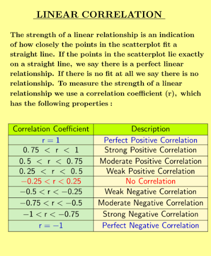
①This example illustrates how randomly generated data can exhibit linear correlation and how to compute the Pearson correlation coefficient (PMCC). ②Key mathematical concepts include correlation analysis, hypothesis testing, and data visualization. ③The construction uses GeoGebra commands RandomUniform for data generation, PMCC for correlation calculation, and Sort, Element, If, TableText for organizing and displaying results. ④Designed for high school and undergraduate statistics or mathematics courses.
GeoGebra Commands & Parameters
RandomUniform(0, 1) → B15RandomUniform(0, 1) → A15RandomUniform(0, 1) → B14RandomUniform(0, 1) → A14RandomUniform(0, 1) → B13RandomUniform(0, 1) → A13RandomUniform(0, 1) → B12RandomUniform(0, 1) → A12RandomUniform(0, 1) → B11RandomUniform(0, 1) → A11RandomUniform(0, 1) → B10RandomUniform(0, 1) → A10RandomUniform(0, 1) → B9RandomUniform(0, 1) → A9RandomUniform(0, 1) → B8RandomUniform(0, 1) → A8RandomUniform(0, 1) → B7RandomUniform(0, 1) → A7RandomUniform(0, 1) → B6RandomUniform(0, 1) → A6RandomUniform(0, 1) → B5RandomUniform(0, 1) → A5RandomUniform(0, 1) → B4RandomUniform(0, 1) → A4RandomUniform(0, 1) → B3RandomUniform(0, 1) → A3RandomUniform(0, 1) → B2RandomUniform(0, 1) → A2RandomUniform(0, 1) → A1PMCC(list1) → aLaTeX(a, true, true) → text1Sort(list2) → list3Sort(list1) → list4Element(list4, 1) → H2Element(list4, 2) → H3Element(list4, 3) → H4Element(list4, 4) → H5Element(list4, 5) → H6Element(list4, 6) → H7Element(list4, 7) → H8Element(list4, 8) → H9Element(list4, 9) → H10Element(list4, 10) → H11Element(list4, 11) → H12Element(list4, 12) → H13Element(list4, 13) → H14Element(list4, 14) → H15PMCC(list6) → cLaTeX(c, true, true) → text4If(c ≟ 1, "Perfect Positive Correlation", If[0.75 < c < 1, "Strong Positive Correlation", If[0.5 < c < 0.75, "Moderate Positive Correlation", If[0.25 < c < 0.5, "Weak Positive Correlation", If[-0.25 < c < 0.25, "NO CORRELATION!", If[-0.5 < c < -0.25, "Weak Negative Correlation", If[-0.75 < c < -0.5, "Moderate Negative Correlation", If[-1 < c < -0.75, "Strong Negative Correlation", If[c ≟ -1, "Perfect Negative Correlation"]]]]]]]]) → SignoTableText({{I1, J1}, {I2, J2}, {I3, J3}, {I4, J4}, {I5, J5}, {I6, J6}, {I7, J7}, {I8, J8}, {I9, J9}, {I10, J10}, {I11, J11}, {I12, J12}, {I13, J13}, {I14, J14}, {I15, J15}}, "c_|h") → text2TableText({{A18, B18}, {A19, B19}, {A20, B20}, {A21, B21}, {A22, B22}, {A23, B23}, {A24, B24}, {A25, B25}, {A26, B26}, {A27, B27}}, "c_|h") → text3
AI Drawing Prompt Reference
Create a set of data points generated randomly and calculate their Pearson correlation coefficient. First, generate 25 random numbers between 0 and 1 for both x and y coordinates, then compute the Pearson correlation coefficient of these points and display the result in LaTeX format. Finally, sort the x and y coordinates and show the coordinates of the first 15 points after sorting.
The prompt above was compiled from the original drawing commands and is for reference only.